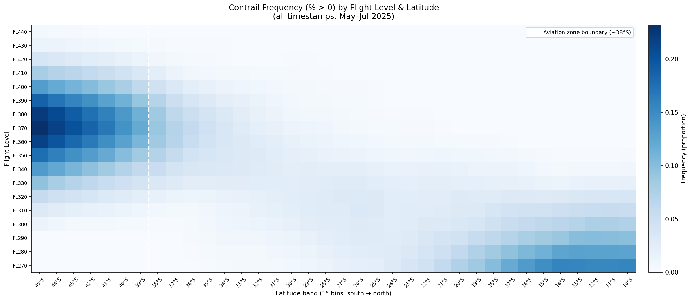
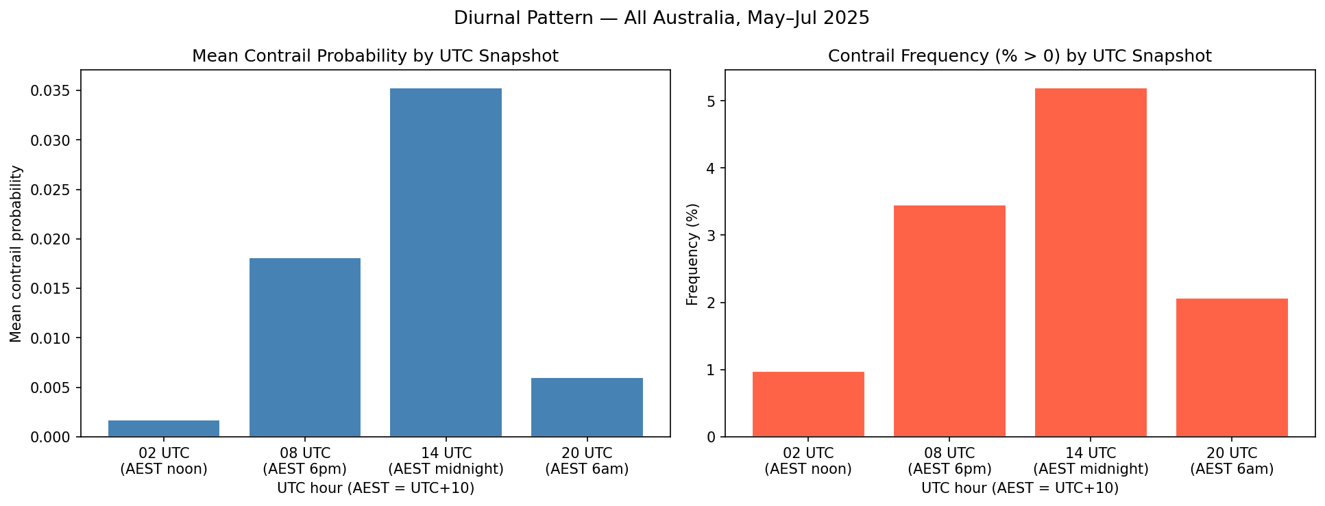
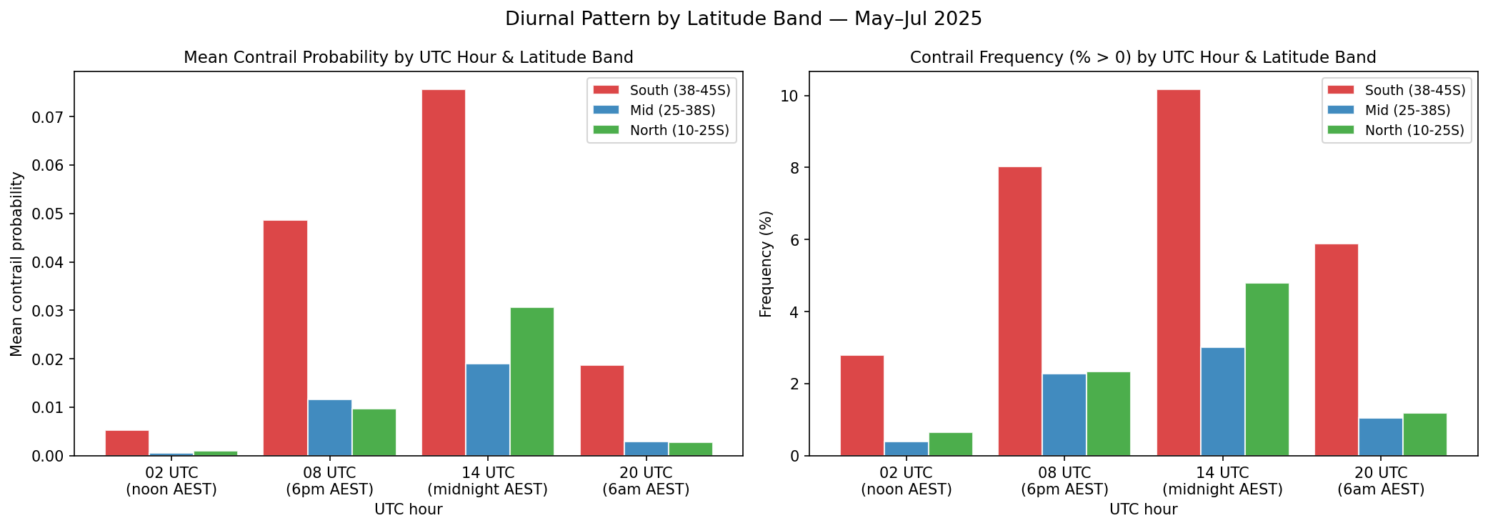
<?xml version="1.0" encoding="utf-8"?><feed xmlns="http://www.w3.org/2005/Atom" ><generator uri="https://jekyllrb.com/" version="3.10.0">Jekyll</generator><link href="https://sidathchandrasena.github.io/feed.xml" rel="self" type="application/atom+xml" /><link href="https://sidathchandrasena.github.io/" rel="alternate" type="text/html" /><updated>2026-10-19T11:49:59+00:00</updated><id>https://sidathchandrasena.github.io/feed.xml</id><title type="html">Sidath Chandrasena</title><subtitle>A portfolio of digital projects by Sidath Chandrasena.</subtitle><author><name>Sidath Chandrasena</name></author><entry><title type="html">Entry 12: Contrails on the Busy SYD-MEL Route</title><link href="https://sidathchandrasena.github.io/2026/10/05/entry-12-mel-to-syd.html" rel="alternate" type="text/html" title="Entry 12: Contrails on the Busy SYD-MEL Route" /><published>2026-10-05T00:00:00+00:00</published><updated>2026-10-05T00:00:00+00:00</updated><id>https://sidathchandrasena.github.io/2026/10/05/entry-12-mel-to-syd</id><content type="html" xml:base="https://sidathchandrasena.github.io/2026/10/05/entry-12-mel-to-syd.html"><![CDATA[<p>Today we’re going to look at another region of interest I found earlier that also happens to be the busiest air route in the English speaking world<sup><a href="#ref1">1</a></sup>: Sydney to Melbourne.</p>

<h4 id="joining-the-dataset">Joining the Dataset</h4>
<p>The range of the data covers 3-26th April 2026. I repeated the same steps as Entry 11 here, except that the contrails data was filtered for the SYD-MEL flight corridor instead of Western Australia. The corridor was defined as the box with longitude between 144 AND 152 and latitude between -38.5 AND -33 and is expected to also capture flights between other major Australian cities, such as Brisbane-Melbourne, Adelaide-Sydney, as well as international traffic.</p>

<p>Next, I filtered the dataset using the <a href="https://github.com/vradarserver/standing-data?tab=CC0-1.0-1-ov-file">standingdata</a> table to check whether each flight had origin/destination as SYD-MEL or MEL-SYD, or was a multi-stop route that included either of the two. In some cases, the route equivalent could not be found in the merge with <a href="https://github.com/vradarserver/standing-data?tab=CC0-1.0-1-ov-file">standingdata</a> and was labeled as unknown, resulting in the following:</p>

<pre><code>route_group
other      20857
unknown     1913
SYD-MEL     1452
Name: count, dtype: int64
</code></pre>

<p>Next, I created a table that labeled a point as a “hit” when CFI &gt; 0.001, with the hit rate representing hits/points * 100. This was separated into SYD-MEL and other flights and unknown, and what percentage of hits each category made.</p>

<table>
  <thead>
    <tr>
      <th>Route group</th>
      <th style="text-align: right">Points</th>
      <th style="text-align: right">Hits</th>
      <th style="text-align: right">Share of hits (%)</th>
      <th style="text-align: right">Hit rate (%)</th>
      <th style="text-align: right">95% CI (±)</th>
    </tr>
  </thead>
  <tbody>
    <tr>
      <td>SYD-MEL</td>
      <td style="text-align: right">1,452</td>
      <td style="text-align: right">34</td>
      <td style="text-align: right">23.13</td>
      <td style="text-align: right">2.34</td>
      <td style="text-align: right">0.78</td>
    </tr>
    <tr>
      <td>Other</td>
      <td style="text-align: right">20,857</td>
      <td style="text-align: right">107</td>
      <td style="text-align: right">72.79</td>
      <td style="text-align: right">0.51</td>
      <td style="text-align: right">0.10</td>
    </tr>
    <tr>
      <td>Unknown</td>
      <td style="text-align: right">1,913</td>
      <td style="text-align: right">6</td>
      <td style="text-align: right">4.08</td>
      <td style="text-align: right">0.31</td>
      <td style="text-align: right">0.25</td>
    </tr>
  </tbody>
</table>

<p>The results show a confidence interval (CI) of around 0.8%, so the true hit rate is somewhere between 1.6-3.1%, while for other flights the hit rate is 0.5% with a CI around 0.1%. This is still an approximation, given that this calculation treats each point as independent, when many points in this data come from the same flight, so the real uncertainty is larger.</p>

<p>The 34 “hits” were collected across 4 days, with most of the hits on 22nd April and then 26th April, so it may just reflect weather events across two days rather than the route itself, and more data is needed to confirm this.</p>

<p>Interestingly, 22nd April was also the day that most at-risk observations were seen over Interior WA in <a href="/2026/07/11/entry-8-examining-interior-wa.html">Entry 8</a> which suggests that a large-scale weather event may have occurred affecting both regions at once. Satellite imagery from 22 April can be used in hindsight to verify whether contrails actually formed over both regions that day.</p>

<p><br /></p>
<h4 id="visualising-the-results">Visualising the Results</h4>
<p>I first wanted to visualise how the SYD-MEL route compared to other flights in contrail at-risk regions.</p>

<p><code>over_under</code> represents whether a group gets more or less “hits” than its share of traffic would predict (share of hits/share of points). A value of 1.0 means the representation is fair, &gt;1 means over-represented and &lt;1 means under-represented.</p>

<table>
  <thead>
    <tr>
      <th>Route group</th>
      <th style="text-align: right">Share of points (%)</th>
      <th style="text-align: right">Share of hits (%)</th>
      <th style="text-align: right">Hit rate (%)</th>
      <th style="text-align: right"><code>over_under</code></th>
    </tr>
  </thead>
  <tbody>
    <tr>
      <td>SYD-MEL</td>
      <td style="text-align: right">5.99</td>
      <td style="text-align: right">23.13</td>
      <td style="text-align: right">2.34</td>
      <td style="text-align: right">3.86</td>
    </tr>
    <tr>
      <td>Other</td>
      <td style="text-align: right">86.11</td>
      <td style="text-align: right">72.79</td>
      <td style="text-align: right">0.51</td>
      <td style="text-align: right">0.85</td>
    </tr>
    <tr>
      <td>Unknown</td>
      <td style="text-align: right">7.90</td>
      <td style="text-align: right">4.08</td>
      <td style="text-align: right">0.31</td>
      <td style="text-align: right">0.52</td>
    </tr>
  </tbody>
</table>

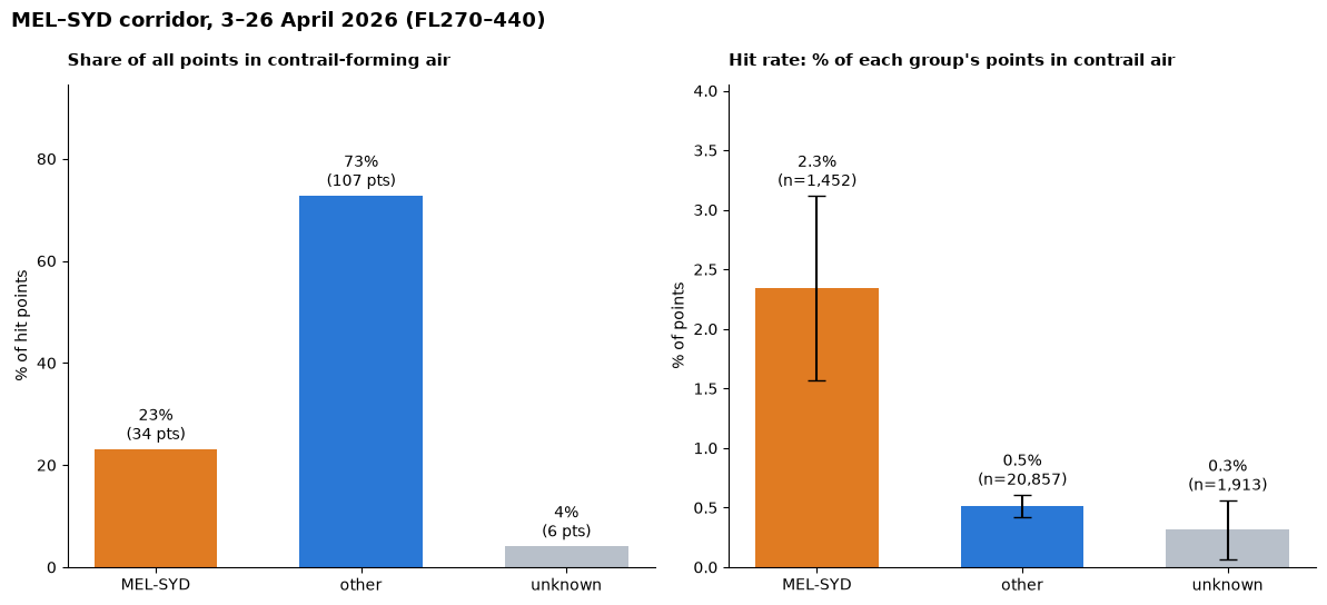
<p>SYD-MEL has an <code>over_under</code> rate of around 3.9x showing a clear over-representation of hits in the data. It is strange that SYD-MEL accounts for 6% of the total points given how busy of a route it is, however it is also important to acknowledge that a lot of other domestic and international routes are captured over the same flight corridor. Also, the sightings in this dataset are not independent because they contain many points for the same flight.</p>

<p>On the left, we have the distribution of the “hits” (places where the point was in at-risk zone) amongst the SYD-MEL, other flights and unknown routes. On the right, we have how much of each group’s sightings were “hits”.</p>

<p><img src="/assets/images/entry_12_mel_syd_hits.png" alt="Comparison of SYD-MEL with other routes in contrail-forming air" /></p>

<p>So we can see that on the left plot, “other” flights account for a large portion of the hits. But that’s also expected given that SYD-MEL is one out of many routes in that corridor. On the right however, we can see that the SYD-MEL route has a much higher amount of “hits”. More analysis will need to be done to discover when this occurs. Is it at cruising altitude?</p>

<p><br /></p>

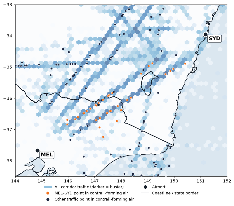
<p>I thought it would be interesting to visually see what all of this looked like on a map.</p>

<p><img src="/assets/images/entry_12_mel_syd_map.png" alt="Map showing SYD-MEL route" /></p>

<p>Two main trajectories can be seen that are reasonably busy between Sydney and Melbourne with several points in contrail-forming air, which points to something valuable for future evaluation. Some questions to be asked here include: are these the most popular trajectories for this route and if so, why? What are some of the implications of changing this route, if it reduces the likelihood of entering contrail-forming areas?</p>

<h4 id="what-would-avoidance-look-like-here">What would avoidance look like here?</h4>

<p>Contrail-forming layers are wide but only a few hundred metres deep<sup><a href="#ref2">2</a></sup>, so climbing or descending around them is easier than flying around them. The Royal Aeronautical Society also describes vertical avoidance as the “most effective route”<sup><a href="#ref3">3</a></sup> but says that in congested airspace, horizontal avoidance might be needed. This would be especially applicable if the routes in the plot above are fixed. Changing the altitude however may be harder in a busy corridor like here where flights all share a limited number of altitudes, and more information will need to be studied to better understand this flight corridor.</p>

<p>There are 2 ways to avoid ice-supersaturated regions or ISSRs: pre-tactical avoidance, which is done before the flight departs, or tactical avoidance, where the avoidance manoeuvers are chosen during the flight<sup><a href="#ref4">4</a></sup>. The latter may pose a greater challenge for the workload of air traffic controllers, a role facing reported staffing shortages in Australia<sup><a href="#ref5">5</a></sup>.</p>

<p><br /></p>
<h4 id="concluding-remarks">Concluding Remarks</h4>
<p>It has been fascinating to compare FIFO services in Interior WA with a much busier part of airspace in Australia. As I look at the above map, I am curious on what makes up the busy air corridor between Sydney and Melbourne. FIFO services tend to be in rural SA, QLD and WA - are they virtually non-existent here? If not, then which group of flights make up the “other” seen in the chart, and are they international or domestic?</p>

<p>Another thing to consider is that my hit rates here counted whether a flight passed through a square where a persistent contrail is likely. However, warming varies between contrails. As mentioned in <a href="/2026/03/09/entry-3-contrail-probabilities-with-respect-to-latitude-altitude-time.html">Entry 3</a>, night-time contrails create more warming than daytime contrails as they only trap heat rather than reflect it. This difference is currently not captured in my analysis, and needs to be covered in the future to better understand which flights have the most impact on the climate. For a start, it would be worth checking whether the hits I found were mostly night-time contrails.</p>

<hr />

<h3 id="references">References</h3>

<div class="references">
  <p><a name="ref1">[1]</a> OAG (2025). <a href="https://www.oag.com/busiest-routes-world-2025">Busiest Routes in the World 2025.</a></p>
  <p><a name="ref2">[2]</a> Jaramillo, P., Kahn Ribeiro, S., Newman, P., et al. (2022), Transport. In <em>Climate Change 2022: Mitigation of Climate Change</em>, Contribution of Working Group III to the Sixth Assessment Report of the Intergovernmental Panel on Climate Change (IPCC) — <a href="https://www.ipcc.ch/report/ar6/wg3/downloads/report/IPCC_AR6_WGIII_Chapter10.pdf">Chapter 10: Transport</a>, p. 1089 (doi:10.1017/9781009157926.012)</p>
  <p><a name="ref3">[3]</a> Royal Aeronautical Society, Greener by Design Specialist Group (2023, April). <a href="https://www.aerosociety.com/media/20657/contrails-and-contrail-management-briefing-paper.pdf">Contrails and contrail management</a> [Briefing paper].</p>
  <p><a name="ref4">[4]</a> Transport &amp; Environment. <a href="https://www.transportenvironment.org/articles/contrail-avoidance">Contrail Avoidance.</a></p>
  <p><a name="ref5">[5]</a> Kennedy, J. (2026, August 10). <a href="https://www.abc.net.au/news/2026-08-10/sydney-airport-near-miss-catherine-king-airservices-staff/107014408">Sydney Airport near miss 'could have been far more serious', air safety boss says.</a> ABC News.</p>
</div>]]></content><author><name>Sidath Chandrasena</name></author><category term="Other" /><summary type="html"><![CDATA[Looking at the merged ADS-B and Contrails dataset in the popular Sydney to Melbourne flight corridor as a comparison to FIFO flights in Interior WA.]]></summary></entry><entry><title type="html">Entry 11: Do FIFO flights enter contrail-forming regions?</title><link href="https://sidathchandrasena.github.io/2026/10/04/entry-11-fifo-and-contrails.html" rel="alternate" type="text/html" title="Entry 11: Do FIFO flights enter contrail-forming regions?" /><published>2026-10-04T00:00:00+00:00</published><updated>2026-10-04T00:00:00+00:00</updated><id>https://sidathchandrasena.github.io/2026/10/04/entry-11-fifo-and-contrails</id><content type="html" xml:base="https://sidathchandrasena.github.io/2026/10/04/entry-11-fifo-and-contrails.html"><![CDATA[<p>Now that I was able to filter the ADS-B dataset to WA and label flights as FIFO and non-FIFO, it’s time to join the dataset with the Google Contrails dataset. From this, I want to now see what percentage of flights that are in the “risk region” for contrail formation.</p>

<h4 id="joining-the-dataset">Joining the Dataset</h4>
<p>The contrails dataset has coordinates that are rounded to 0.25, so the ADS-B data had to first be rounded so there could be a match. So this was done to the longitude and latitude columns. Flight level was also rounded to the nearest 10 to match the contrails dataset. This was also done for the timestamp column, which in the contrails table only records results for each multiple of 6 (UTC 00, 06, 12, 18), so each result is rounded to one of these four times to match. The ADS-B data was then filtered between FL270 and FL440 as this was the altitude range the Contrails API covers.</p>

<p>Next, the rounded timestamp column was filtered in the ADS-B dataset to make sure it matches the timestamps in the contrails dataset.</p>

<p>Then the rounded matching columns in the ADS-B dataset were renamed to match the contrails dataset and a left merge was performed.</p>

<p>The <code>fillna()</code> command was run on <code>contrails</code> for rows where there was no match, as this indicates a contrail forcing index of zero. A sighting is counted as “at-risk” when CFI &gt; 0.001.</p>

<p>Next, I created a new variable called <code>local_date</code> to convert the timestamp from UTC to Perth time.</p>

<p>Next, I imported the FIFO dataset labeled from last entry and then performed an inner merge to get this merged table to have labeling. This left the resulting table with only Australian airlines, with the FIFO/non-FIFO label attached to every sighting of each flight.</p>

<p><br /></p>
<h4 id="visualising-the-results">Visualising the Results</h4>
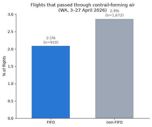
<p>I first wanted to see how many of the flights in the dataset that pass through contrail-forming air are FIFO or non-FIFO by percentage.</p>

<p><img src="/assets/images/entry_11_contrail_distribution.png" alt="Flights that passed through contrail-forming air FIFO vs non-FIFO" /></p>

<p>The plot shows the share of non-FIFO and FIFO flights that passed through contrail-forming air (if any of its sightings over WA was in a cell with CFI &gt; 0.001).</p>

<p>This revealed 2.1% of FIFO flights (n = 910) passing through contrail-forming air compared to 2.9% of non-FIFO flights (n = 1672). Considering that 2.1% of 910 is around 19 flights and 2.9% of 1672 is around 48 flights, a two proportion z-test on Jupyter Notebooks using the math module gets a p-value of 0.23, which is not statistically significant and shows that the data doesn’t provide enough evidence of a true difference between the two. So more data is needed to understand this gap.</p>

<p><br /></p>

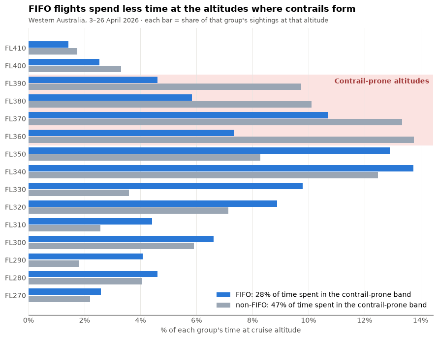
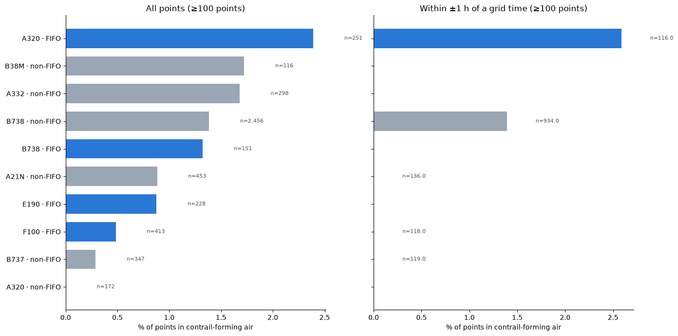
<p>The next plot shows the altitude distribution among FIFO and non-FIFO flights. The right-hand plot shows when you filter out observations that were rounded to beyond 1 hour of the recorded time (given contrails data) was every 6 hours, this accounts for a big disparity between the observation and time. However, on the other hand, this means a significantly smaller number of observations).</p>

<p><img src="/assets/images/entry_11_altitude_distribution.png" alt="FIFO vs non-FIFO by Altitude" /></p>

<p>As seen above, non-FIFO flights dominate at altitudes beyond FL340 and contrail-prone altitudes as well. Maybe due to FIFO flights having small aircraft? Let’s verify that.</p>

<p><br />
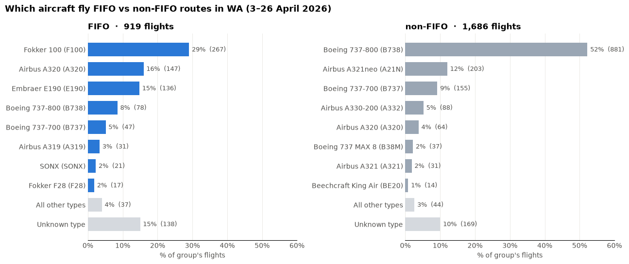
<img src="/assets/images/entry_11_aircraft_distribution.png" alt="FIFO vs non-FIFO routes by frequency" /></p>

<p>Let’s compare the difference between the cruising altitude of a Fokker 100 with a Boeing 737-800. Fokker 100 has a maximum operating altitude of 35,000 ft<sup><a href="#ref1">1</a></sup> while Boeing 737-800 has a maximum operating altitude of 41,000 ft<sup><a href="#ref2">2</a></sup>. While the Fokker 100’s maximum altitude is still within the above “contrail-prone” altitude grid, it helps with understanding why FIFO flights may represent a smaller portion of the flights in the region of interest.</p>

<p><br />
Now let’s look at the aircraft distribution amongst FIFO and non-FIFO flights in at-risk regions.</p>

<p><img src="/assets/images/entry_11_fleet_distribution.png" alt="Comparing Aircraft Type FIFO vs non-FIFO" /></p>

<p>What I find to be interesting here is the big difference in the number of observations between the top and bottom bar of FIFO and non-FIFO, despite being the same aircraft. Also the Boeing 737-MAX at second from top, and then Boeing 737-800 below, is that to do with the increased adoption of MAX aircraft in domestic Australia?</p>

<p>Perhaps this should be taken with some skepticism, however, as the right-hand plot demonstrates that when the data is filtered to within one hour of the observation, it seems that the diversity in aircraft type is significantly reduced, with n = 6136 reduced to n = 2259 meaning that 37% of points were kept.</p>

<p><br /></p>
<h4 id="concluding-remarks">Concluding Remarks</h4>
<p>These findings can take us in many directions. What I am most curious about from today’s results is identifying which FIFO aircraft are responsible for those results in the contrail risk zone. I am guessing that they are those flights in those planes that match the common planes for non-FIFO services, such as Airbus A320s and Boeing 737-800s. From this I wonder: what prompts a FIFO service or charter to be done in a large passenger jet as opposed to a small one? What are those routes? What are the implications of a shift in aircraft operation on the mining industry and the FIFO workforce?</p>

<p>I plan to take a small break from looking at FIFO work to compare this to another region of interest identified in a previous entry: the infamous Sydney-Melbourne route.</p>

<hr />

<h3 id="references">References</h3>

<div class="references">
  <p><a name="ref1">[1]</a> European Union Aviation Safety Agency (2022). <a href="https://www.easa.europa.eu/en/downloads/7450/en">Type-Certificate Data Sheet No. EASA.A.037 for Fokker F28</a> (Issue 08; F28 Mark 0100 section).</p>
  <p><a name="ref2">[2]</a> European Union Aviation Safety Agency (2025). <a href="https://www.easa.europa.eu/en/downloads/7297/en">Type-Certificate Data Sheet No. IM.A.120 for Boeing 737</a> (Issue 29; 737 Next Generation sections).</p>
</div>]]></content><author><name>Sidath Chandrasena</name></author><category term="Other" /><summary type="html"><![CDATA[Bringing in the contrails dataset with the labeled FIFO vs non-FIFO ADS-B dataset of Australian aircraft over Western Australia to identify whether FIFO flights enter contrail-prone regions.]]></summary></entry><entry><title type="html">Entry 10: A More Accurate Picture of FIFO Flights</title><link href="https://sidathchandrasena.github.io/2026/10/03/entry-10-a-more-accurate-picture-of-fifo-flights.html" rel="alternate" type="text/html" title="Entry 10: A More Accurate Picture of FIFO Flights" /><published>2026-10-03T00:00:00+00:00</published><updated>2026-10-03T00:00:00+00:00</updated><id>https://sidathchandrasena.github.io/2026/10/03/entry-10-a-more-accurate-picture-of-fifo-flights</id><content type="html" xml:base="https://sidathchandrasena.github.io/2026/10/03/entry-10-a-more-accurate-picture-of-fifo-flights.html"><![CDATA[<p>Last entry provided a glimpse into how Australia’s mining industry plays a big role in our aviation industry. I also found this graphic<sup><a href="#ref1">1</a></sup> which shows a pretty cool visualisation of how FIFO flights look in the grand scale of things.</p>

<p>In my last analysis, I used some big assumptions to label flights as FIFO vs non-FIFO based on carrier. However, since then, I have come to see that this is not a great way to estimate if a flight is a FIFO service or not. While I don’t plan to do anything particularly as complex as creating a model, I want to use this entry to get a more accurate depiction of FIFO scheduling and then hopefully use this dataset in my next entry with my Contrails data, which has continued to grow with my cron job.</p>

<p><br /></p>
<h3 id="filtering-data">Filtering Data</h3>

<p>This time, I used my ADSB data and filtered it using state boundaries to filter the dataset to Western Australia instead of the whole Australian continent.</p>

<p><br /></p>
<pre><code class="language-python">wa = states.loc[
    (states["admin"] == "Australia") &amp; (states["name"] == "Western Australia"),
    "geometry",
].iloc[0]

gdf = gpd.GeoDataFrame(df, geometry=gpd.points_from_xy(df.longitude, df.latitude), crs="EPSG:4326")
df_wa = gdf[gdf.within(wa)]
</code></pre>

<p><br /></p>

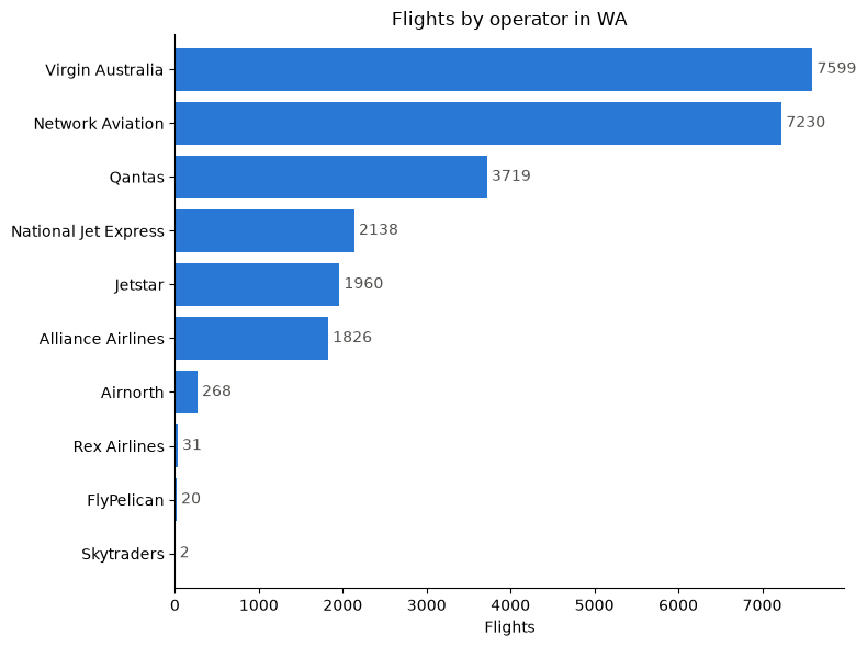
<p>I initially thought of using the registration number of the plane to filter data, but noticed that this can be inconsistent with the operating airline (e.g. if an airline sells the plane to another company). I also realised that callsign is not a great way to distinguish a carrier, as this seems to conflate airlines with its subsidiaries (e.g. Qantas + Network Aviation + QantasLink).</p>

<p>I decided to filter using icao24 which are 24-bit addresses using Australia’s hex range, which is 7C0000–7FFFFF<sup><a href="#ref2">2</a></sup>. I also made sure to keep the earliest entry for that aircraft to remove duplicate entries.</p>

<p>I then merged this with OpenSky data on the icao24 column which gave me information such as: operator, owner, and aircraft.</p>

<p><img src="/assets/images/entry_10_flights_by_carrier.png" alt="Frequency of flights by operator in WA" /></p>

<p>Interestingly, QLK callsign for Qantaslink is completely absent from WA due to the QantasLink brand being completely operated by Network Aviation there. Virgin Australia Regional Airlines and Virgin Australia are also indistinguishable by callsign.</p>

<p><br /></p>
<h3 id="how-to-best-distinguish-fifo-vs-non-fifo">How to best distinguish FIFO vs non-FIFO?</h3>
<p>After some confusion with operator codes, I decided that for the scope of this task, I would use flight number and origin/destination to determine if a flight was FIFO or non-FIFO.</p>

<p><br /></p>
<h4 id="flight-number-rules">Flight Number Rules</h4>
<p>On major airlines:</p>

<p><strong>Virgin Australia:</strong> Flights VA9000 to VA9999 are operated by Virgin Australia Regional Airlines and are listed as charter services<sup><a href="#ref3">3</a></sup> which I will take to be FIFO services for this exercise.</p>

<p><strong>Qantas:</strong> QF1600–QF1999 are FIFO services<sup><a href="#ref4">4</a></sup> and QF2700–2735, QF2770–2775 and QF6590–6599 are all Network Aviation flight numbers<sup><a href="#ref5">5</a></sup>, which can be considered as FIFO here.</p>

<p><strong>Jetstar:</strong> All flights can be labeled non-FIFO as it is a LCC carrier</p>

<p><strong>Alliance Airlines:</strong> Could not find a clear designation of flight number being FIFO or not. Considering it’s described as Australia’s major FIFO operator, I am going to label all as FIFO despite it being a simplification.</p>

<p><strong>Rex (Regional Express):</strong> all FIFO flights are operated via National Jet Express, so I labelled all ZL/RXA flights as non-FIFO<sup><a href="#ref6">6</a></sup>.</p>

<p><br /></p>
<h4 id="origindestination-filtering">Origin/Destination Filtering</h4>
<p>I used <a href="https://github.com/vradarserver/standing-data#CC0-1.0-1-ov-file">standingdata</a> on Github’s repo containing callsigns and their corresponding route (origin-destination) and then joined that with my dataset.</p>

<p>I located the airports of several confirmed mine sites using the ICAO codes: “YCHK”, “YFDF”, “YANG”, “YBGD”, “YWGA”, “YIBO”, “YGIA”, “YSOL”, “YEWA”</p>

<p><br />
<br />
After doing both of these filtering actions, I got the following using pandas crosstab.</p>

<p>Note that the “unknown” label was applied when the standingdata merge did not result in a match for the callsign so the origin or destination of a flight could not be determined, nor could the FIFO status be later determined from the flight number. “Unlabelled” is used when there was a flight number with a matching origin/destination but none of the flight number airline-specific rules were applied to them. I couldn’t determine a flight number rule for Network Aviation to classify as FIFO/non-FIFO, which is a weakness as most flights are likely to be FIFO but outside of my mine-site airport list. “none” represents cases where the flight callsign failed to match with an airline in my list from Wikipedia of Australian airlines, which are mostly small Australian-registered aircraft which are private, business and small charter flights.</p>

<p>There are definitely a lot of limitations in the dataset, but let’s see if there’s an improvement to the plots:</p>

<pre><code class="language-text">fifo_or_non_fifo      FIFO  non-FIFO  unknown  unlabelled
airline
Airnorth                 0         0       55         214
Alliance Airlines     1852         0        0           0
FlyPelican               0         0       21           0
Jetstar                  0      1979        0           0
National Jet Express  2157         0        0           0
Network Aviation      1747         0      667        4900
Qantas                  88      3572        0           0
Rex Airlines             0        31        0           0
Skytraders               0         0        2           0
Virgin Australia      2824      4789        0           0
none                     0         0     4522           0
</code></pre>

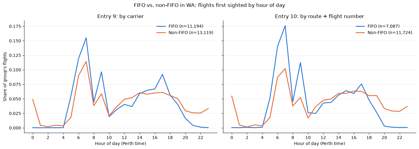
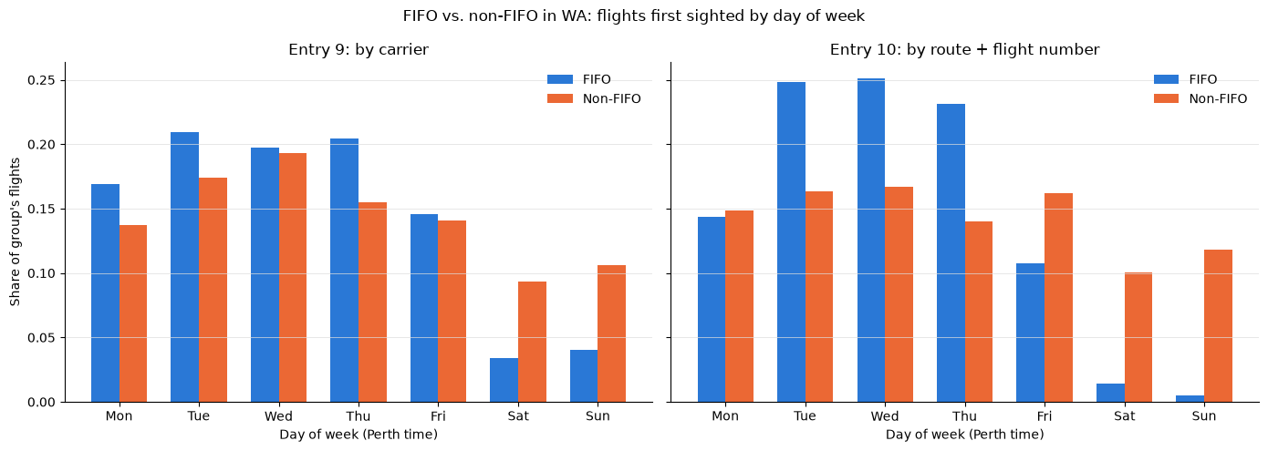
<p>Next, I plotted my plots from Entry 9 with the newly filtered and more accurate Entry 10 data to compare FIFO vs non-FIFO flights in day of week and time of day.</p>

<p><img src="/assets/images/entry_10_comparison_time_of_day.png" alt="FIFO vs non-FIFO in WA by hour of day compared with Entry 9" /></p>

<p>The effects are much more pronounced for FIFO flights, with a large majority of flights occurring early in the day or around 5pm. This is explained as the “morning wave”, where workers arrive early to get to the site and work their 12-hour days by mid-morning<sup><a href="#ref7">7</a></sup>. The rise in the afternoon is explained by workers completing their shifts and returning to Perth where they commute home<sup><a href="#ref8">8</a></sup>.</p>

<p>The human factors element here is important for any future contrail-avoidance scheme. Maisey et al. <sup><a href="#ref7">7</a></sup> found that shift start times earlier than 06:00 can result in significant sleep loss and reduced alertness throughout the day, which can pose accident and health risks. The implications of this are that shifting FIFO departures to avoid contrail-forming air would need to balance accounting for its effect on workers with costs to companies such as weekend penalty rates.</p>

<p><img src="/assets/images/entry_10_comparison_day_of_week.png" alt="FIFO vs non-FIFO in WA by day of week compared with Entry 9" /></p>

<p>Compared to Entry 9, there is a more visible split in proportion of weekend flights for FIFO compared to non-FIFO Saturday through Monday and then more FIFO flights occurring on weekdays. Weekend flights are uncommon for FIFO perhaps because weekends result in penalty rates for crew (higher expenses) and there are limited flights in regional areas on weekends.</p>

<p><br /></p>

<p>It is exciting to work with the data directly on Jupyter Notebooks using Pandas but I don’t want to go down a rabbithole in refining FIFO vs non-FIFO classification! I look forward to using this dataset next with the contrails dataset.</p>

<p><br /></p>
<h3 id="references">References</h3>
<div class="references">
  <p><a name="ref1">[1]</a> r/perth (Reddit). <a href="https://www.reddit.com/r/perth/comments/14vnz06/air_traffic_around_australia_eight_hours/">Air traffic around Australia, eight hours.</a></p>
  <p><a name="ref2">[2]</a> AirLabs. <a href="https://airlabs.co/icao-24-bit-address">ICAO 24-bit address.</a></p>
  <p><a name="ref3">[3]</a> Hong Kong Airlines. <a href="https://www.hongkongairlines.com/en_CN/FFP/earn/airlines_partner-VA">Airline partner: Virgin Australia.</a></p>
  <p><a name="ref4">[4]</a> Australian Frequent Flyer. <a href="https://www.australianfrequentflyer.com.au/qantas-flight-numbers/">Qantas flight numbers.</a></p>
  <p><a name="ref5">[5]</a> Qantas Group. <a href="https://www.qantas.com/en-au/where-we-fly/network-aviation">Network Aviation.</a></p>
  <p><a name="ref6">[6]</a> Regional Express (Rex) (2022, September 30). <a href="https://www.rex.com.au/BlobViewer/BlobViewer.aspx?attachtype=MR&amp;filename=6F6254563278466A6A474853692B6D756A31643639342F66716361714562457647676D6C7467465836774C6178415073444F78563470434E4B4B656F7533394B4E503158526358357A4F5A7769676F3646484E6F43673D3D">Rex finalises purchase of National Jet Express</a> [Media release].</p>
  <p><a name="ref7">[7]</a> Maisey, G., Cattani, M., Devine, A., Lo, J., Fu, S. C., &amp; Dunican, I. C. (2022). <a href="https://doi.org/10.1016/j.apergo.2021.103617">Digging for data: How sleep is losing out to roster design, sleep disorders, and lifestyle factors.</a> <em>Applied Ergonomics</em>, 99, 103617.</p>
  <p><a name="ref8">[8]</a> Smithies, T. D., Vincent, G. E., Ferguson, S. A., Maisey, G., Fraser, H., &amp; Dunican, I. C. (2026). <a href="https://doi.org/10.1093/annweh/wxag007">Drilling down on roster design: comparing fly-in fly-out roster patterns in the West Australian mining industry.</a> <em>Annals of Work Exposures and Health, 70</em>(2), wxag007.</p>
</div>]]></content><author><name>Sidath Chandrasena</name></author><category term="Other" /><summary type="html"><![CDATA[Improving the filtered ADS-B dataset to classify Australian flights over Western Australia as FIFO vs non-FIFO using origin/destination and flight numbers.]]></summary></entry><entry><title type="html">Entry 9: Exploring FIFO Charter Flights</title><link href="https://sidathchandrasena.github.io/2026/09/12/entry-9-exploring-fifo-charter-flights.html" rel="alternate" type="text/html" title="Entry 9: Exploring FIFO Charter Flights" /><published>2026-09-12T00:00:00+00:00</published><updated>2026-09-12T00:00:00+00:00</updated><id>https://sidathchandrasena.github.io/2026/09/12/entry-9-exploring-fifo-charter-flights</id><content type="html" xml:base="https://sidathchandrasena.github.io/2026/09/12/entry-9-exploring-fifo-charter-flights.html"><![CDATA[<p>Last time, my discoveries into Interior WA, an area I knew little about, revealed a large number of flights for FIFO work. In this entry, I plan to take a glance at what FIFO work is, and how it’s represented in my growing dataset.</p>

<p><br /></p>
<h3 id="what-is-fifo-work">What is FIFO work?</h3>

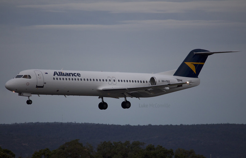
<p>Growing up in South Australia, I was familiar with the term FIFO meaning “fly-in, fly-out” and its association with the mining industry with places such as Olympic Dam listed as destinations on small regional flights. In terms of those who work in the FIFO industry, what comes to mind is people who wear hardhats and hi-vis vests, but I imagined all sorts of people connected to the industry including site engineers, tradesmen and executives.</p>

<figure>
  <img src="/assets/images/entry_9_fifo_plane.jpg" alt="Alliance Airlines Fokker 100 VH-FKK" />
  <figcaption>"Alliance Airlines | Fokker 100 VH-FKK" by Luke McConville is licensed under CC BY-NC-ND 2.0. To view a copy of this licence, visit https://creativecommons.org/licenses/by-nc-nd/2.0/?ref=openverse.</figcaption>
</figure>

<p>Some preliminary research reveals that FIFO work takes place primarily in QLD and WA as these states have a lot of mining sites and involves specialists coming into the site to do work over a rostered period. Some of the roles include engineers, electricians, security guards, nurses, chefs, etc<sup><a href="#ref1">1</a></sup>.</p>

<p>I was curious why people would choose to repeatedly commute instead of relocating, which could provide a lot of opportunities for the area near the mining site. An article by Windle and Rolfe<sup><a href="#ref2">2</a></sup> revealed that salaries would need to be increased significantly for someone to relocate instead of FIFO work. It seems that the Australian mining industry is very reliant on this kind of work.</p>

<p>From one article<sup><a href="#ref3">3</a></sup>, I found some examples of the typical rosters FIFO workers take on:</p>
<ul>
  <li>8/6 (work eight days, have six days off)</li>
  <li>2/1 (works two weeks, one week off)</li>
  <li>4/2 (work four weeks, then two weeks off)</li>
  <li>Even time: equal time on-site and off-site</li>
</ul>

<p>To gain a better idea of what FIFO scheduling looks like, I decided to look at my own dataset. In Entry 8, we can see that there was a carrier called “Network Aviation”, which I found is a Perth-based carrier that provides scheduled and charter services for FIFO workers.<sup><a href="#ref4">4</a></sup></p>

<p><br /></p>
<h3 id="exploring-fifo-scheduling-with-pandas">Exploring FIFO Scheduling with Pandas</h3>

<p>My goal is to see how scheduling or flight frequency differs between regional FIFO carriers and the major carriers flying between cities.</p>

<p>In my Jupyter notebook, I imported my ADSB.fi traffic data into a Pandas dataframe. I then filtered the data to Australian airspace using a NaturalEarth polygon, and filtered to only Australian carriers using the list of Australian airlines and their ICAO codes on Wikipedia.</p>

<p>I realised that several factors would need to be considered to determine whether a flight was a FIFO flight: terminal, flight number and some airlines may do both FIFO and intercity routes (e.g. Virgin Australia).</p>

<p>For now, what I chose to do is to pick three airlines that do largely intercity routes (Qantas, Virgin Australia, Jetstar) and three carriers that largely operate FIFO services (Network Aviation, National Jet Express and Alliance Airlines).</p>

<p>The resulting dataframe contained columns including: <code>callsign</code>, <code>airline</code>, <code>latitude</code>, <code>longitude</code>, <code>flight_level</code>, <code>carrier_group</code>.</p>

<p><br /></p>
<h4 id="plot-1-fifo-vs-non-fifo---hour-of-day">Plot 1: FIFO vs non-FIFO - Hour of Day</h4>
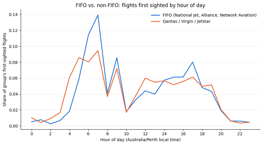
<p>For the first plot, I wanted to view how FIFO vs non-FIFO flights frequency differs in time of day, keeping in mind that ADSB.fi data is real-time traffic rather than scheduled departure. So I grabbed the earliest seen point of each flight and got the following plot.</p>

<p><img src="/assets/images/entry_9_fifo_hour_of_day.png" alt="FIFO vs non-FIFO flight frequency by hour of day" /></p>

<p>FIFO flights compared to non-FIFO peak around 5am and 5pm Perth local time. Non-FIFO flights represent a higher proportion of all flights before 5am, between 10am-2pm and 6-8pm. This seems to align well with many (paywalled) articles online depicting how extremely early FIFO flights have led to some health concerns over poor sleep quality and risks of car accidents to and from the airport. One example of an article that explores this is Maisey et al<sup><a href="#ref5">5</a></sup>.</p>

<p><br /></p>
<h4 id="plot-2-fifo-vs-non-fifo---day-of-the-week">Plot 2: FIFO vs non-FIFO - Day of the Week</h4>
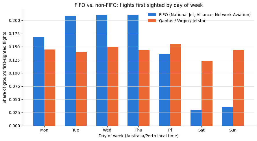
<p>I also wanted to see whether the above mentioned rosters may be reflected when plotted against the days of the week.</p>

<p><img src="/assets/images/entry_9_fifo_day_of_week.png" alt="FIFO vs non-FIFO flight frequency by day of week" /></p>

<p>Here we can see that FIFO flights consistently make a higher proportion of air traffic in Australian airspace Tues-Thurs, and then at the end of the week (Fri-Sun), commercial flights make up a much higher proportion.</p>

<p>Looking at information online on FIFO flights and which days on the week they are: one website<sup><a href="#ref6">6</a></sup> mentions how you fly out at the beginning of the week, typically Sunday or Monday (which contrasts with my dataset which seems to be Monday or Tuesday) and return in two weeks or so repeatedly on a 2:1 schedule. There may be other factors that contribute to the above plot’s shape, such as whether workers fly in their own time or in company time, as this would factor into things such as penalty rates on weekends.</p>

<p><br /></p>

<h3 id="reflections">Reflections</h3>
<p>Learning about FIFO work from an aviation point of view was intriguing and I see it as something to further look into. Today’s analysis also raises some questions and thoughts:</p>

<ul>
  <li>Which FIFO routes are more susceptible to crossing regions likely to form contrails?</li>
  <li>How does aircraft type affect contrail formation, given that FIFO flights are considerably smaller than intercity flights? <strong>(see <a href="/2026/10/04/entry-11-fifo-and-contrails.html">Entry 11</a>)</strong>.</li>
  <li>How does the frequency of FIFO flights vary seasonally?</li>
</ul>

<p><br /></p>

<h3 id="references">References</h3>

<div class="references">
  <p><a name="ref1">[1]</a> Cummings Economics (2013). <a href="https://www.cummings.net.au/pdf/recent/J2681FIFOWorkforceCairnsRegion.pdf">FIFO workforce in the Cairns region</a> (Report J2681).</p>
  <p><a name="ref2">[2]</a> Windle, J., &amp; Rolfe, J. (2013). <a href="https://doi.org/10.1016/j.resourpol.2012.10.006">Using discrete choice experiments to assess the preferences of new mining workforce to commute or relocate to the Surat Basin in Australia.</a> <em>Resources Policy</em>, 38(2), 169–180.</p>
  <p><a name="ref3">[3]</a> Tim D Smithies, Grace E Vincent, Sally A Ferguson, Gemma Maisey, Holly Fraser, Ian C Dunican, <a href="https://doi.org/10.1093/annweh/wxag007">Drilling down on roster design: comparing fly-in fly-out roster patterns in the West Australian mining industry</a>, Annals of Work Exposures and Health, Volume 70, Issue 2, March 2026, wxag007</p>
  <p><a name="ref4">[4]</a> Qantas Group. <a href="https://www.qantas.com/en-au/where-we-fly/network-aviation">Network Aviation.</a></p>
  <p><a name="ref5">[5]</a> Maisey, G., Cattani, M., Devine, A., Lo, J., Fu, S. C., &amp; Dunican, I. C. (2022). <a href="https://doi.org/10.1016/j.apergo.2021.103617">Digging for data: How sleep is losing out to roster design, sleep disorders, and lifestyle factors.</a> <em>Applied Ergonomics</em>, 99, 103617.</p>
  <p><a name="ref6">[6]</a> Programmed by Persol. <a href="https://skilled.programmed.com.au/working-fifo-australia-pay-rosters-lifestyle-what-to-expect/">Working FIFO in Australia: Pay, Rosters, Lifestyle and What to Expect.</a></p>
</div>]]></content><author><name>Sidath Chandrasena</name></author><category term="Other" /><summary type="html"><![CDATA[Researching what fly-in, fly-out (FIFO) work is and filtering ADS-B traffic data to visualise and better understand FIFO flight scheduling.]]></summary></entry><entry><title type="html">Entry 8: Examining Interior WA</title><link href="https://sidathchandrasena.github.io/2026/07/11/entry-8-examining-interior-wa.html" rel="alternate" type="text/html" title="Entry 8: Examining Interior WA" /><published>2026-07-11T00:00:00+00:00</published><updated>2026-07-11T00:00:00+00:00</updated><id>https://sidathchandrasena.github.io/2026/07/11/entry-8-examining-interior-wa</id><content type="html" xml:base="https://sidathchandrasena.github.io/2026/07/11/entry-8-examining-interior-wa.html"><![CDATA[<p>Some regions identified in past entries included the Bass Strait and Tasman Sea. These were areas where climate conditions made contrail formation likely, but also where air traffic was high enough. For the Tasman Sea, we can imagine flights between Australia and NZ, and Bass Strait includes flights from the Australian mainland to Tasmania.</p>

<p>One region that was also discovered last entry was Interior WA. Today’s entry will take a look at this in more detail from a purely data point of view.</p>

<hr />

<h4 id="the-data">The Data</h4>
<p>While entry 7 had eight days’ worth of data that aligns between ADSB air traffic and Google Contrails data, for today’s analysis, we have data spanning across 24 days between 3-26 April, 2026.</p>

<p>The ADS-B dataset contained over 9,000 entries. From this, we came up with a yes/no flag on a single aircraft sighting. If at that moment, a plane is inside a grid cell with CFI&gt;0.001, the sighting is counted as “at-risk”. A single plane can have multiple counts inside an at-risk cell, and unlike the previous entry, it is not a compound score of the CFI and air traffic.</p>

<p>In code, this was written as follows:</p>

<pre><code class="language-python"># contrail_prob = the CFI in the grid cell each sighting was
#                 snapped to (0 if the plane was in clear air)
exposure["in_risk"] = exposure["contrail_prob"] &gt; 0.001   # &gt; 0.001  →  at-risk (True / False)
n_at_risk = exposure["in_risk"].sum()                     # count the True's
</code></pre>

<p>To narrow down the dataset to WA, we created a bounding box around the clustered at-risk observations seen in Entry 7, the coordinates being: <code>112.5–122.5° / -34.5° to -27.5°</code>.</p>

<p>Our data can now be summarised as:</p>

<table>
  <thead>
    <tr>
      <th> </th>
      <th>Value</th>
    </tr>
  </thead>
  <tbody>
    <tr>
      <td>Window</td>
      <td>3–26 April 2026 (24 days, date-matched)</td>
    </tr>
    <tr>
      <td>Aircraft observations in the box</td>
      <td><strong>9,776</strong></td>
    </tr>
    <tr>
      <td>Observations inside active contrail air</td>
      <td><strong>136 (1.39%)</strong></td>
    </tr>
    <tr>
      <td>Distinct at-risk aircraft</td>
      <td>87</td>
    </tr>
    <tr>
      <td>Days with at least one at-risk flight</td>
      <td><strong>9 of 24</strong></td>
    </tr>
  </tbody>
</table>

<h4 id="at-risk-observations-across-the-24-days">At-Risk Observations Across the 24 Days</h4>
<p>Our first plot shows the amount of at-risk observations across the 24-days.</p>

<figure>
  <img src="/assets/images/entry_8_timeline.png" alt="At-risk flights per day over interior WA" />
  <figcaption>At-risk flights per day over interior WA</figcaption>
</figure>

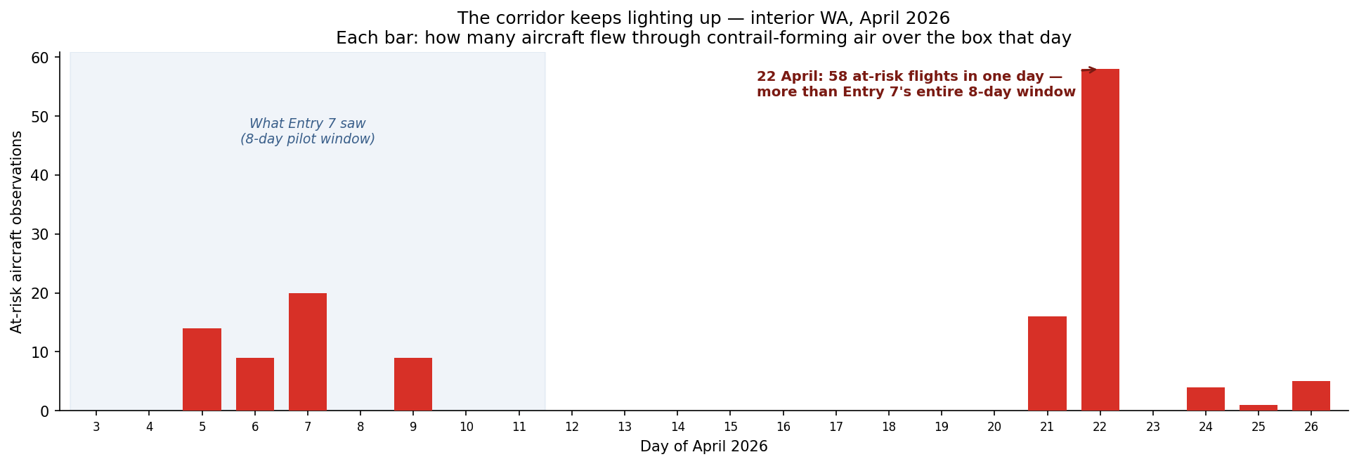
<p>What’s interesting to observe is that there are lots of days where at-risk observations are little to zero, and there are several days with notable “spikes”. The most prominent example is April 22, which accounts for 43% of all observations from our dataset.</p>

<p>The spike is not caused by increased air traffic, as air traffic remains steady throughout and 22 April was an ordinary day in terms of air traffic. It would be interesting to look into other factors that may have caused this, such as humidity and temperatures that day.</p>

<h4 id="at-what-height-did-airplanes-get-caught-in-contrail-forming-air">At What Height Did Airplanes Get Caught in Contrail-Forming Air?</h4>
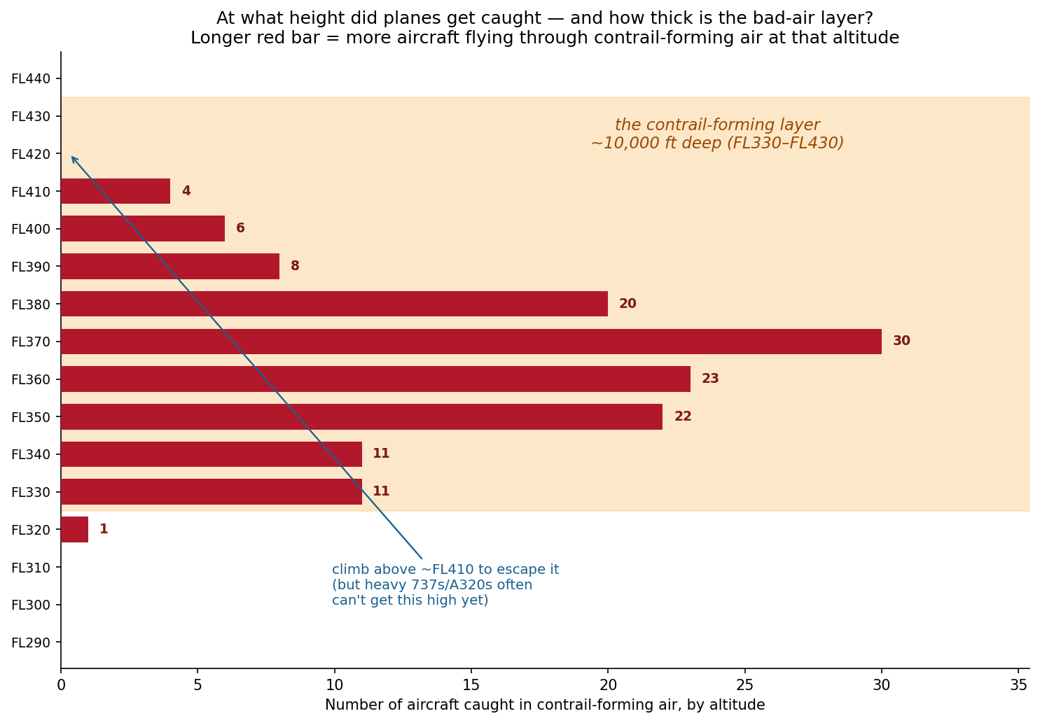
<p>The altitudes range from around FL330-FL410, which spans around 10,000 ft deep. There is a noticeable peak at around FL370, which is standard narrowbody cruise altitude. This is some food for thought, as it may pose a challenge for any altitude avoidance strategies.</p>

<p>If contrail-forming air can be anywhere across this range of altitudes, avoiding it with altitude-avoidance strategies can also result in an increase in fuel burn. However, researchers at Imperial College London<sup><a href="#ref1">1</a></sup> and the University of Cambridge<sup><a href="#ref2">2</a></sup> found that the warming avoided more than offset this fuel burn.</p>

<figure>
  <img src="/assets/images/entry_8_altitude.png" alt="Altitude distribution of at-risk flights over interior WA" />
  <figcaption>How deep the contrail-forming layer is, by altitude</figcaption>
</figure>

<h4 id="map-of-observations-by-contrail-forcing-index">Map of Observations by Contrail Forcing Index</h4>
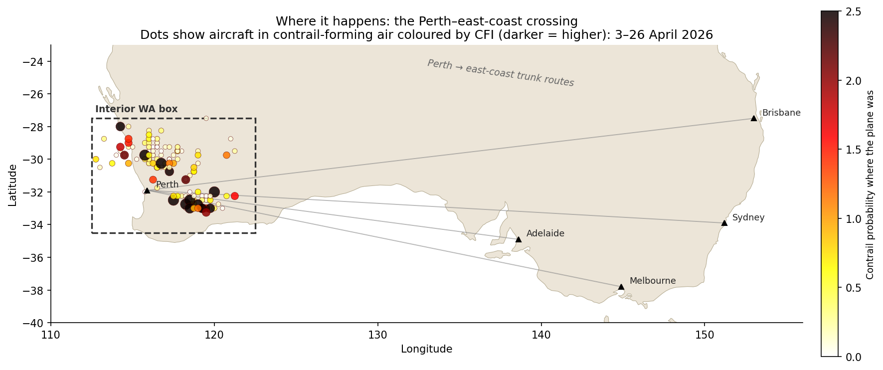
<p>Below is a way to visualise everything from a bigger picture point of view with routes out of Perth visible.</p>

<figure>
  <img src="/assets/images/entry_8_corridor_map_2.png" alt="Map of the Perth to east-coast corridor over interior WA" />
  <figcaption>Where it happens — the Perth to east-coast corridor</figcaption>
</figure>

<p>Looking at the data more closely, it is not one route responsible for most of the data points, but it is distributed well across multiple routes. The busiest callsign appears four times.</p>

<table>
  <thead>
    <tr>
      <th>Operator</th>
      <th style="text-align: right">At-risk obs</th>
      <th>What they are</th>
    </tr>
  </thead>
  <tbody>
    <tr>
      <td><strong>Virgin Australia</strong> (VOZ)</td>
      <td style="text-align: right">41</td>
      <td>Perth–east-coast trunk (737)</td>
    </tr>
    <tr>
      <td><strong>Network Aviation</strong> (NWK)</td>
      <td style="text-align: right"><strong>21</strong></td>
      <td><strong>Qantas-owned FIFO mining charters within WA</strong></td>
    </tr>
    <tr>
      <td><strong>Qantas</strong> (QFA)</td>
      <td style="text-align: right">18</td>
      <td>Perth–east-coast trunk (737/A330)</td>
    </tr>
    <tr>
      <td>Jetstar (JST/JTE)</td>
      <td style="text-align: right">14</td>
      <td>Low-cost domestic + Perth–Singapore</td>
    </tr>
    <tr>
      <td>Everyone else combined</td>
      <td style="text-align: right">~42</td>
      <td>Mostly foreign carriers transiting Perth</td>
    </tr>
  </tbody>
</table>

<p>One interesting observation above is “Network Aviation” at second place, which are all of the FIFO (fly in, fly out) operations between Perth and remote WA for mining work.</p>

<p>Below is also the distribution by aircraft type:</p>

<table>
  <thead>
    <tr>
      <th>Aircraft type</th>
      <th style="text-align: right">At-risk obs</th>
    </tr>
  </thead>
  <tbody>
    <tr>
      <td>B738 (737-800)</td>
      <td style="text-align: right">45</td>
    </tr>
    <tr>
      <td>A320</td>
      <td style="text-align: right">19</td>
    </tr>
    <tr>
      <td>A21N / A319 (neo + classic)</td>
      <td style="text-align: right">14</td>
    </tr>
    <tr>
      <td><strong>F100 (Fokker 100 — FIFO)</strong></td>
      <td style="text-align: right"><strong>9</strong></td>
    </tr>
    <tr>
      <td>E190</td>
      <td style="text-align: right">8</td>
    </tr>
    <tr>
      <td>B788 / B38M / A332 / A388 …</td>
      <td style="text-align: right">the widebody + regional tail</td>
    </tr>
  </tbody>
</table>

<p>Out of the three regions of interest in Australian airspace, Interior WA intrigues me a lot because it is an interesting case where there is an entire industry that requires people to fly short-haul constantly for their commute. More to come in my next post to unpack what FIFO is.</p>

<hr />

<h3 id="references">References</h3>

<div class="references">
  <p><a name="ref1">[1]</a> Teoh, R., Schumann, U., Majumdar, A., &amp; Stettler, M. E. J. (2020). <a href="https://doi.org/10.1021/acs.est.9b05608">Mitigating the climate forcing of aircraft contrails by small-scale diversions and technology adoption.</a> <em>Environmental Science &amp; Technology</em>, 54(5), 2941–2950.</p>
  <p><a name="ref2">[2]</a> Smith, J. R., Grobler, C., Hodgson, P. J., et al. (2026). <a href="https://doi.org/10.1038/s41467-026-68784-8">The climate opportunities and risks of contrail avoidance.</a> <em>Nature Communications</em>, 17, 2092.</p>
</div>]]></content><author><name>Sidath Chandrasena</name></author><category term="Other" /><summary type="html"><![CDATA[Looking at a bigger set of matched contrails and ADS-B data to reveal where contrail hotspots may be in Western Australia in April 2026.]]></summary></entry><entry><title type="html">Entry 7: When Real Flights Meet Contrail Skies</title><link href="https://sidathchandrasena.github.io/2026/04/12/entry-7-ads-b-meets-contrail-data.html" rel="alternate" type="text/html" title="Entry 7: When Real Flights Meet Contrail Skies" /><published>2026-04-12T00:00:00+00:00</published><updated>2026-04-12T00:00:00+00:00</updated><id>https://sidathchandrasena.github.io/2026/04/12/entry-7-ads-b-meets-contrail-data</id><content type="html" xml:base="https://sidathchandrasena.github.io/2026/04/12/entry-7-ads-b-meets-contrail-data.html"><![CDATA[<p>Entries 5 and 6 had limited ADS-B (air traffic) data, resulting in the flight traffic data and contrail data being from different time periods: we had to overlay March 2026 OpenSky flight traffic data on winter 2025 contrail grids.</p>

<p>In this post, both datasets cover the same eight-day window of <strong>3-11 April 2026</strong>, which will give us a more accurate picture of the relationship between contrail formation likelihood and air traffic in Australian skies.</p>

<h3 id="datasets">Datasets</h3>
<h4 id="dataset-a-contrail_grids">Dataset A: <code>contrail_grids</code></h4>

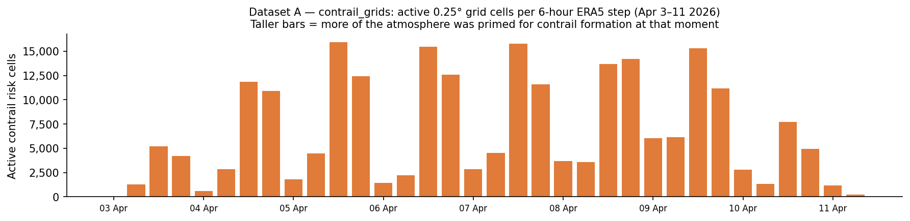
<p>This is the Google Contrails API data. It splits Australia’s airspace into squares about 28 km wide. Every 6 hours, a weather model assesses whether a contrail would form if a plane flew through there with a continuous CFI float value between 0 and 4. My dataset only retains squares with a value greater than 0.001.</p>

<p>The dataset is in Autumn 2026, and a lot smaller in size compared to previous datasets during the Winter 2025 timeframe. The difference in results could be explained by the different climate conditions across seasons in the Southern Hemisphere, but the two datasets also cover different years and lengths of time, so they aren’t exactly comparable.</p>

<p>To summarise Dataset A:</p>

<table>
  <thead>
    <tr>
      <th>Attribute</th>
      <th>Value</th>
    </tr>
  </thead>
  <tbody>
    <tr>
      <td><strong>Source</strong></td>
      <td>Google Contrails API</td>
    </tr>
    <tr>
      <td><strong>Period</strong></td>
      <td>3–11 April 2026</td>
    </tr>
    <tr>
      <td><strong>Temporal resolution</strong></td>
      <td>6-hour intervals (00:00, 06:00, 12:00, 18:00 UTC)</td>
    </tr>
    <tr>
      <td><strong>Spatial resolution</strong></td>
      <td>0.25° × 0.25° grid (≈28 km at Australian latitudes)</td>
    </tr>
    <tr>
      <td><strong>Altitude range</strong></td>
      <td>FL270–FL440 (18 levels)</td>
    </tr>
    <tr>
      <td><strong>Total rows stored</strong></td>
      <td>234,817 cells (CFI &gt; 0.001) across 36 snapshots</td>
    </tr>
  </tbody>
</table>

<p>The figure below shows how each bar represents one 6-hourly forecast snapshot.</p>

<figure>
  <img src="/assets/images/entry_7_dataset_a_overview.png" alt="Dataset A overview" />
  <figcaption>Bar Plot of Contrail Grid Dataset</figcaption>
</figure>

<h4 id="dataset-b---flight_snapshots">Dataset B - <code>flight_snapshots</code></h4>

<p>Dataset B uses ADSB.fi, a free alternative to OpenSky that provides community-driven and crowdsourced air traffic data.</p>

<p>The data was collected using a Github workflow titled <code>collect-flights.yml</code>, which runs a script called <code>collect_flights_adsb.py</code> every 30 minutes. ADSB.fi then returns a big JSON blob with one aircraft per entry. The script filters to only accept aircraft above FL200 (20,000 ft), making sure they are airborne.</p>

<table>
  <thead>
    <tr>
      <th>Attribute</th>
      <th>Value</th>
    </tr>
  </thead>
  <tbody>
    <tr>
      <td><strong>Source</strong></td>
      <td>ADS-B.fi open API (12 tiling circles)</td>
    </tr>
    <tr>
      <td><strong>Period</strong></td>
      <td>3–11 April 2026</td>
    </tr>
    <tr>
      <td><strong>Poll frequency</strong></td>
      <td>Every ~30 minutes (472 polls over the window)</td>
    </tr>
    <tr>
      <td><strong>Total rows</strong></td>
      <td>30,150</td>
    </tr>
    <tr>
      <td><strong>Unique aircraft</strong></td>
      <td>1,560 distinct ICAO hex addresses</td>
    </tr>
    <tr>
      <td><strong>Altitude filter</strong></td>
      <td>FL200 and above only</td>
    </tr>
  </tbody>
</table>

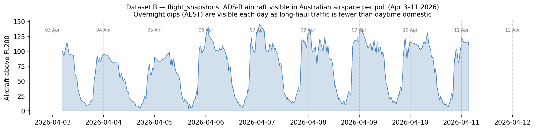
<p>The plot below illustrates Dataset B, air traffic over time in Australian skies. The troughs represent AEST night (~ UTC 12:00-22:00) when fewer aircraft are at cruise altitude. Daily peaks coincide with the busy late-morning domestic period.</p>

<p><img src="/assets/images/entry_7_dataset_b_overview.png" alt="Dataset B overview" /></p>

<hr />

<h3 id="lets-combine-both-plots-together">Let’s combine both plots together.</h3>
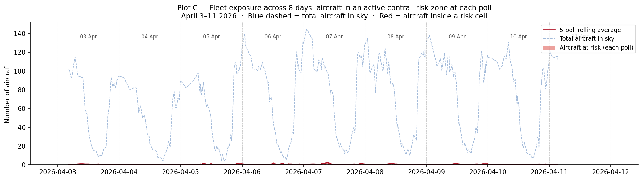
<p>This way, we can investigate: how much of all the aircraft in Australian skies is exposed to contrail-risk regions at one time? Each snapshot captures how many aircraft were inside an active contrail risk cell at a point in time. The blue dashed-line shows the total aircraft in the sky at each poll and the red line shows how many of those aircraft were at risk.</p>

<p>For most of the 8-day window, the red and blue lines are far apart with only few aircraft (around 0-3) inside a contrail risk cell compared to up to 140 aircraft in the sky. So exposure was a small fraction of traffic throughout with no clear spike on any specific day.</p>

<p><img src="/assets/images/entry_7_exposure_timeseries.png" alt="Fleet exposure over time" /></p>

<hr />

<h3 id="where-does-this-risk-occur-on-an-australian-map">Where does this risk occur (on an Australian map)?</h3>

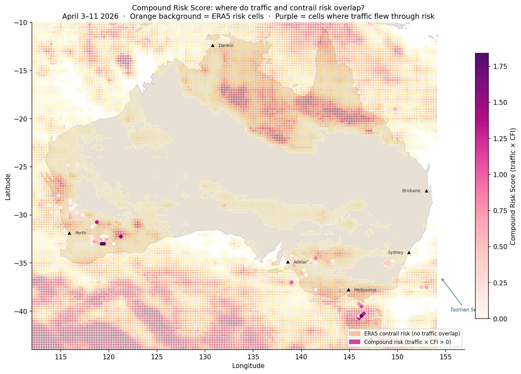
<p>The heatmap placed over the map of Australia below shows the <strong>Compound Risk Score (CRS) = total aircraft observations in that cell x mean contrail forcing index</strong>, meaning cells where aircraft flew through active contrail risk.</p>

<p>There are some notable clusters of purple - the Western Australia interior and Bass Strait. The Tasman Sea to the right also showed some intersection of contrail risk and flight traffic to a lesser extent than seen earlier in Entry 5.</p>

<p><img src="/assets/images/entry_7_geographic_risk_2.png" alt="Compound risk geography" /></p>

<hr />

<h3 id="what-time-of-day-is-contrail-risk-the-highest">What time of day is contrail risk the highest?</h3>
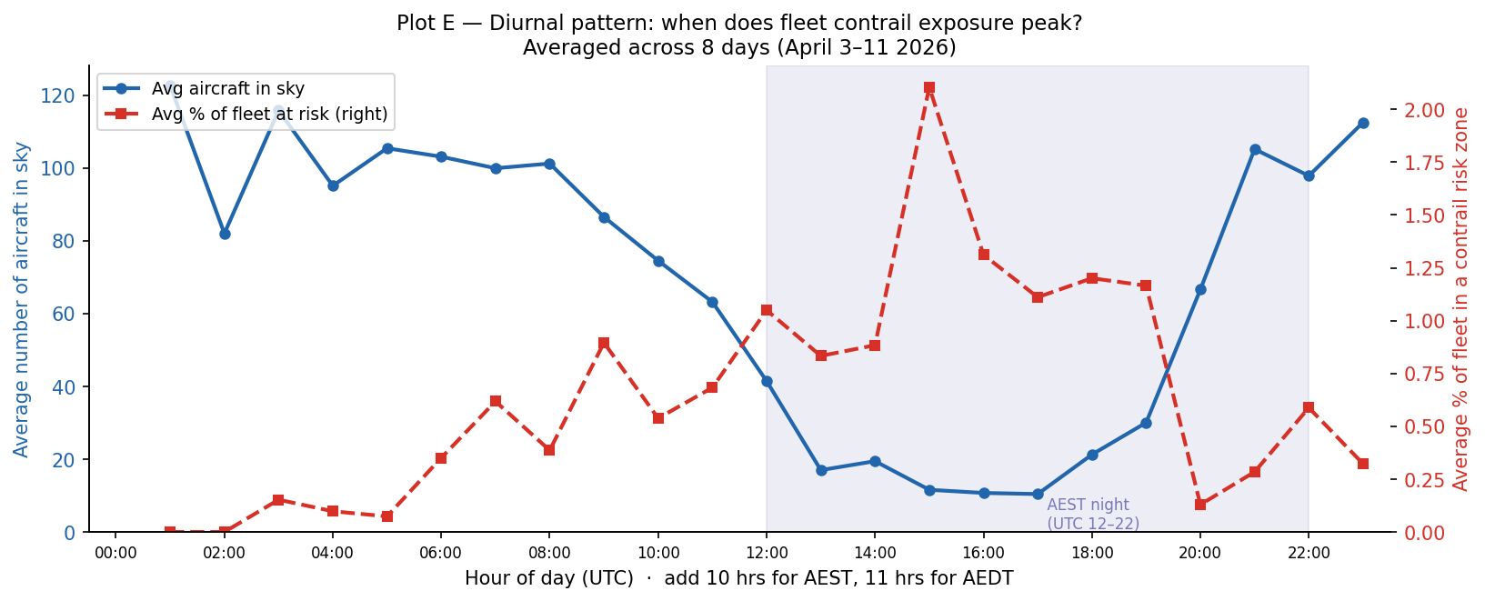
<p>The below plot combines 8 days’ worth of data into one single 24-hour UTC clock that identifies at what time contrail exposure peaks.</p>

<p><img src="/assets/images/entry_7_diurnal.png" alt="Diurnal pattern" /></p>

<p>The blue line (left axis) shows the average number of aircraft in the sky at each UTC hour. This shows a low at AEST night and a high across the daytime domestic period (peaking around UTC 0:00, which is ~10:00 AEST).</p>

<p>The red dashed line (right axis) shows the average percentage of active fleet inside a contrail risk zone at each UTC hour. This peaks at 15 UTC (01:00 AEST), so the middle of Australian overnight with a low at 01-02 UTC (11:00-12:00 AEST). This matches what was observed earlier in Entry 3.</p>

<p>The key finding here is that the hours with the most air traffic (UTC 22:00-02:00, morning to midday AEST) are not the most prone to contrail exposure, but rather the quieter overnight window.</p>

<hr />

<h2 id="questions--takeaways">Questions + Takeaways</h2>
<p><strong>Takeaways:</strong></p>
<ul>
  <li>
    <p>In addition to the Bass Strait and Tasman Sea, another area of interest identified for contrail formation risk is the interior of WA.</p>
  </li>
  <li>
    <p>The overnight window is when the highest risk of contrail formation occurs rather than the hours when there is the most air traffic.</p>
  </li>
</ul>

<p><strong>Food for thought for the next entry:</strong></p>

<ul>
  <li>
    <p>How does this dataset from April compare to other months?</p>
  </li>
  <li>
    <p>What weather data can we use to understand the changes in at-risk aircraft?</p>
  </li>
  <li>
    <p>What causes the WA interior, Bass Strait and Tasman Sea to have a higher risk of contrail formation?</p>
  </li>
</ul>]]></content><author><name>Sidath Chandrasena</name></author><category term="Other" /><summary type="html"><![CDATA[This time, contrail data is matched with ADS-B flight traffic data covering the same window in Autumn 2026 to see where busy skies and contrail-prone areas overlap.]]></summary></entry><entry><title type="html">Entry 6: Charting Australia’s Domestic Skies</title><link href="https://sidathchandrasena.github.io/2026/04/03/entry-6-domestic-flight-routes.html" rel="alternate" type="text/html" title="Entry 6: Charting Australia’s Domestic Skies" /><published>2026-04-03T00:00:00+00:00</published><updated>2026-04-03T00:00:00+00:00</updated><id>https://sidathchandrasena.github.io/2026/04/03/entry-6-domestic-flight-routes</id><content type="html" xml:base="https://sidathchandrasena.github.io/2026/04/03/entry-6-domestic-flight-routes.html"><![CDATA[<p>Last post, I used a very limited amount of ADS-B data to get a glimpse into how contrail formation in winter intersects with air traffic inside Australia. Despite how limited the ADSB data was, it showed how contrail formation likelihood may not align directly with where the air traffic is, and identified the Bass Strait as a region to be investigated further, where there was a reasonable amount of air traffic and contrail forcing index.</p>

<p>OpenSky’s free tier ran out of credits quite fast, so I decided to use a Github Action to collect a snapshot of Australian airspace every 15 minutes. It will take a week to collect a good amount of data, so this post is what I am doing while waiting for that.</p>

<hr />

<p>In Australia, BITRE (Bureau of Infrastructure, Transport and Regional Economics) provides a free, downloadable dataset of monthly domestic aviation statistics with the total number of flights and seats for that month. In today’s post, I plan to look at domestic flight routes, particularly the busiest ones, and evaluate them with the contrail risk data.</p>

<p>Entry 5 found from some limited OpenSky data that flights were observed to mostly be at FL320–FL400 in Australian skies. A quick search online at flight reports shows a cruising altitude from SYD-MEL ranging from FL330 to FL400.</p>

<hr />
<h3 id="how-this-analysis-was-done">How this analysis was done</h3>

<p><strong>Transparent Sheet:</strong> Used 28km squares over a map of Australia and coloured each square by how often the atmosphere at cruising altitude (FL320-400) contains the conditions for contrails to form and persist. Dark squares indicate where the atmosphere is prone to contrail formation.</p>

<p><strong>Great Circle Paths:</strong> on a globe, the shortest path between two points is a slight curve known as a “great circle”. For short routes that curve is almost identical to a straight line on a flat map, while for longer routes it arcs more noticeably. I go along each great circle and record which grid squares it passes through, treating the whole route as if it were at cruise, which may overstate the exposure at airports where planes would be climbing or descending.</p>

<p><strong>The BITRE dataset:</strong> Contains monthly domestic aviation statistics with every city pair in Australia. We downloaded all 12 months of 2024 and added them up to get annual flight counts. For each route, multiplied contrail risk along the great circle path by the annual flight count resulting in a total annual exposure score that indicates how contrail-forming the route’s geography is with its flying frequency.</p>

<p>In summary, our dataset looks like this:</p>

<table>
  <thead>
    <tr>
      <th>Source</th>
      <th>Detail</th>
    </tr>
  </thead>
  <tbody>
    <tr>
      <td><strong>Contrail risk grid</strong></td>
      <td>Uses 2 models: ML-based model and Contrail Cirrus Prediction (CoCiP), FL320–FL400, May–July 2025, 239 timestamps, 25,521 grid cells at 0.25° resolution</td>
    </tr>
    <tr>
      <td><strong>Flight traffic</strong></td>
      <td>BITRE monthly domestic aviation statistics, all 12 months of 2024, 62 city pairs with known airport coordinates</td>
    </tr>
    <tr>
      <td><strong>Path model</strong></td>
      <td>Great circle arcs sampled at 150 points; assumes all points to be at cruise altitude (within Australian bounding box)</td>
    </tr>
  </tbody>
</table>

<p>Note there are some limitations. First, great circle paths are not exact. Second, BITRE provides a seats-per-flights figure which we can assume aircraft size. For flights with low passenger size, they are likely to be operated by turboprops which have a much lower cruising altitude. This causes the exposure score to overstate actual contrail risk, which is important to keep in mind.</p>

<hr />
<h3 id="routes-vs-contrail-risk">Routes vs Contrail Risk</h3>
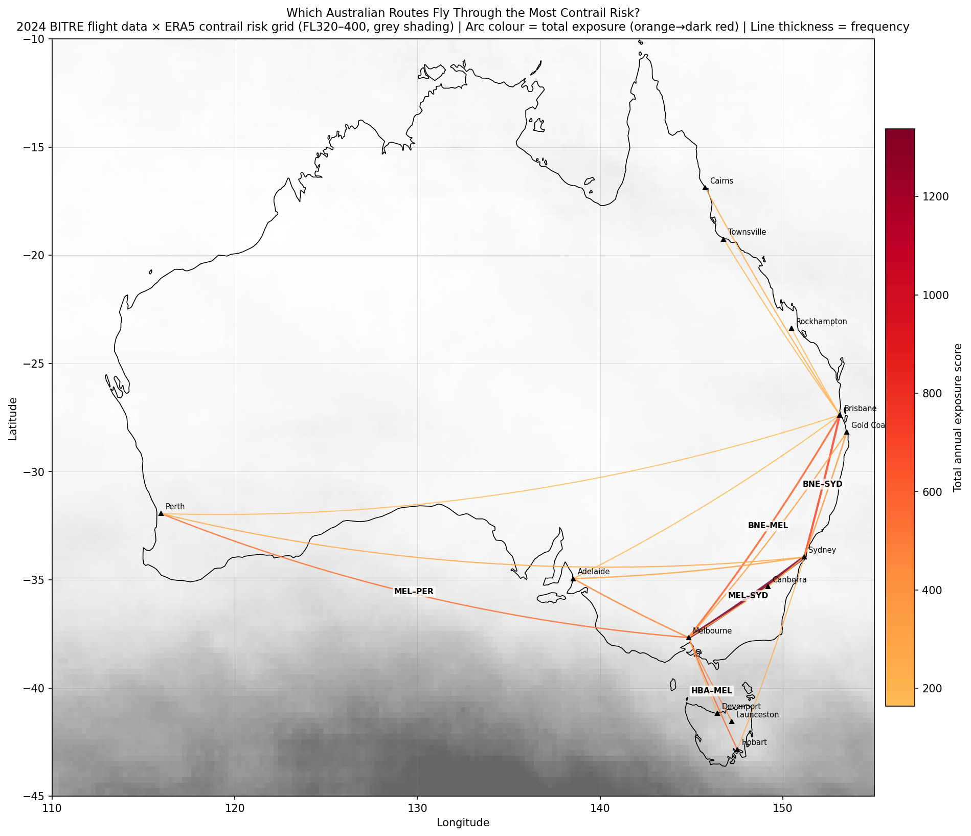
<p>The top 20 routes by total annual exposure over the contrail risk grid. Arc colour indicates exposure score, with dark red being high and thickness indicates flight frequency.</p>

<p><img src="/assets/images/entry_6_route_map.png" alt="Route Map" /></p>

<p>The map reveals that almost all the action is focused on southeastern Australia and the Bass Strait/Tasmania corridor. Northern Territory is largely unlit because the atmosphere there is low-risk relatively as indicated by the white shading compared to the South. The SYD-MEL route as expected is visually dominant due to high air traffic but HBA-MEL stands out because the route crosses through the highest-risk cells in the entire dataset.</p>

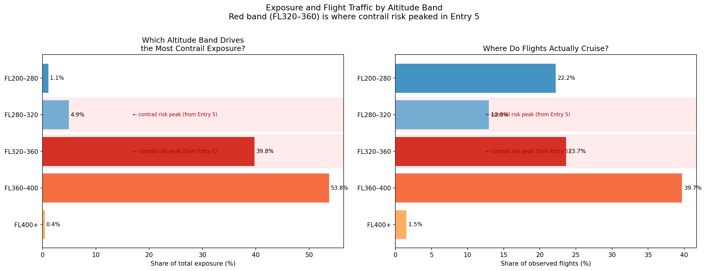
<p><img src="/assets/images/entry_6_band_breakdown.png" alt="Contrail Risk by Altitude Band" /></p>

<h3 id="busy-routes-vs-risky-zones">Busy Routes vs Risky Zones</h3>
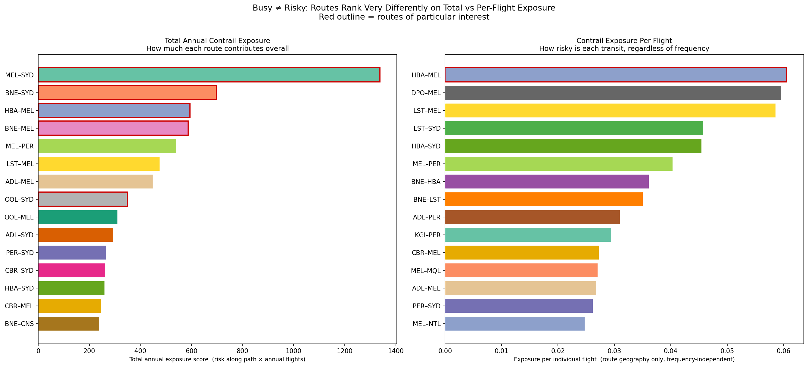
<p>Left: top 15 routes by total annual exposure. Right: top 15 routes by exposure per flight (frequency taken out of the equation).</p>

<p><img src="/assets/images/entry_6_exposure_comparison.png" alt="Busy Routes vs Risky Zones" /></p>

<p>The Melbourne to Sydney route is Australia’s biggest contrail contributor overall with an exposure score of 1,337 and 55,624 flights in 2024. On the right plot however it can be seen that its per flight score puts it around 8th. So it’s not necessarily a contrail-prone route, but given that it is one of the busiest domestic routes in the world, it accumulates more exposure than any other route.</p>

<p>Hobart to Melbourne is the most contrail-prone route per individual flight with a per-flight risk score of 0.0605, which is 2.5x higher than SYD-MEL’s 0.024. Each HBA-MEL flight crosses the Bass Strait on a path that runs almost directly over the cluster of highest-risk cells seen in previous posts. It ranks 3rd in total exposure despite carrying only around a sixth of SYD-MEL’s traffic.</p>

<h3 id="what-factors-determine-contrail-exposure">What Factors Determine Contrail Exposure?</h3>
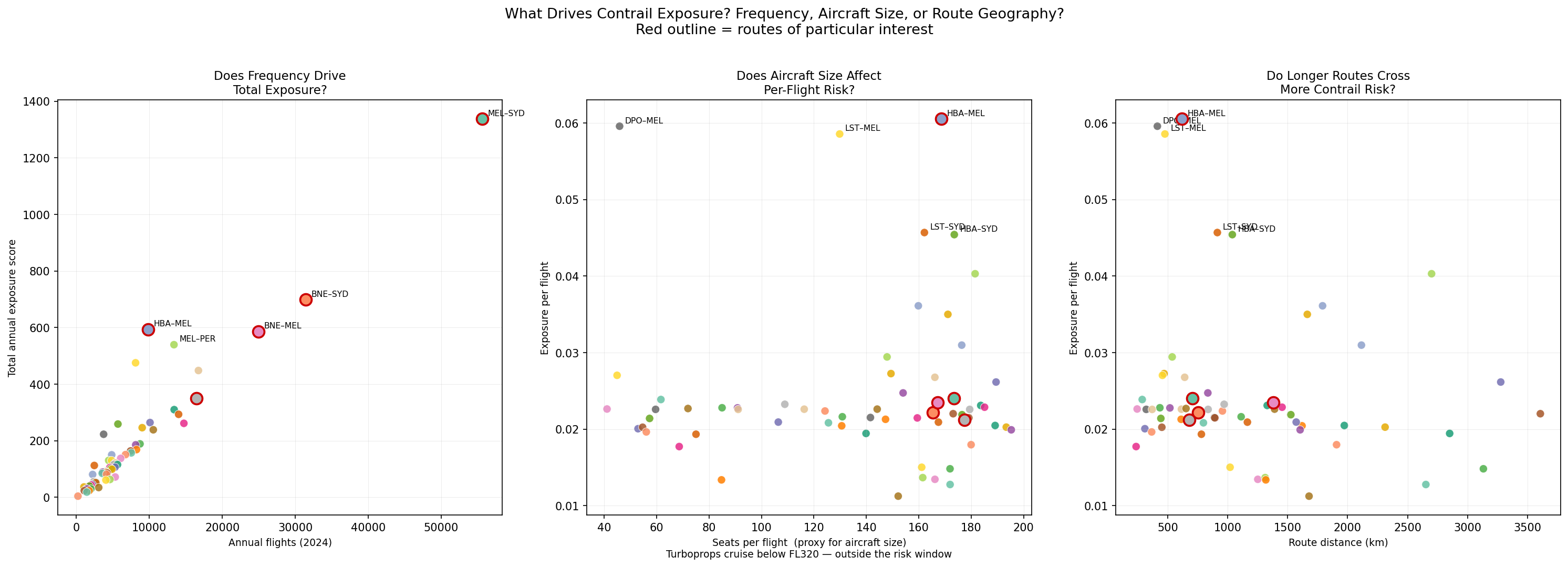
<p>To look into this question, 3 scatter plots were generated examining the roles of frequency, seats per flight (aircraft size) and route distance.</p>

<p><img src="/assets/images/entry_6_factors.png" alt="Factors Driving Contrail Exposure" /></p>

<p>Plot 1 shows a strong correlation between annual flight count and total exposure. This matches what we saw with SYD-MEL flights where when a route is flown more often, total exposure accumulates. However, this relationship is not purely linear, with an example being HBA-MEL which sits above the trend line because the per-flight risk is so much higher than average.</p>

<p>In Plot 2, as mentioned earlier, routes with few seats (&lt;70) tend to be turboprop planes which results in some scattered results because they actually fly at much lower altitudes below the risk window. The highest per-flight scorers all have 100+ seats, which indicates that they are jet-operated routes. Routes like DPO-MEL score high in exposure but have low seat numbers per flight (turboprop) so the high score reflects Bass Strait geography rather than a real contrail exposure.</p>

<p>Plot 3 shows a weak positive trend between route distance and per-flight risk. The per-flight risk score is calculated by averaging the risk of squares a route crosses, so the distance of the route doesn’t cause risk to increase, what matters more is the skies the route passes through. For example, routes to Perth are long but have a moderate per-flight risk as their track crosses the low-risk, arid interior while Tasmanian routes are shorter but score high because every km of their cruise phase is over the Bass Strait risk corridor.</p>

<h2 id="main-takeaways">Main Takeaways</h2>
<p>While waiting on ADSB data to load, we were able to get some interesting information using BITRE data along with our Contrails and OpenSky data.</p>

<p>With what we have, we can see examples of how contrail formation risk appears in different ways. In some cases, it is high-risk and low-traffic, and in other cases, it can be low-risk and high-traffic.</p>

<p>The ADS-B data, when loaded, will provide more supporting information. Particularly to answer questions such as whether the actual paths match the great circles, or if every flight on the same route hits the same risk cells? Some other considerations for future posts include looking at turboprop flights at lower altitudes, and looking at how data at other times in the year (seasonality) affects things.</p>]]></content><author><name>Sidath Chandrasena</name></author><category term="Other" /><summary type="html"><![CDATA[Taking a look at Australia's domestic flight network with government data to find out which routes carry the most traffic, and how do they align with contrail-prone skies?]]></summary></entry><entry><title type="html">Entry 5: Adding in Flight Data</title><link href="https://sidathchandrasena.github.io/2026/03/15/entry-5-adding-in-flight-data.html" rel="alternate" type="text/html" title="Entry 5: Adding in Flight Data" /><published>2026-03-15T00:00:00+00:00</published><updated>2026-03-15T00:00:00+00:00</updated><id>https://sidathchandrasena.github.io/2026/03/15/entry-5-adding-in-flight-data</id><content type="html" xml:base="https://sidathchandrasena.github.io/2026/03/15/entry-5-adding-in-flight-data.html"><![CDATA[<p>In previous posts, we looked purely at contrail formation index based on altitude and coordinates. In this post, we’re going to add a flight traffic layer to move from “where do contrails form” to “where do contrails form where there is also high air traffic?”.</p>

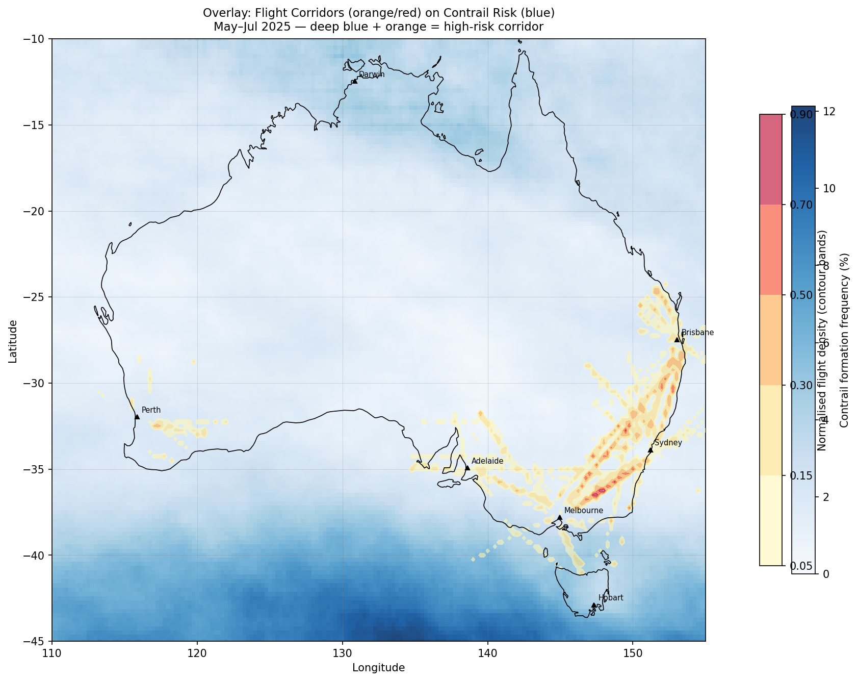
<p>The data needed to find this out is ADS-B data, which provides insights into flight traffic. To get ADS-B data, I created an account on OpenSky. However, a standard account restricts queries to the last hour and I need researcher access to match the May-Jul 2025 window that matches the Contrails data timeframe. For now, assuming that flight routes remain largely stable year-round, I can use existing data to get some insights. Using this, I got four insightful plots.</p>

<h3 id="plot-1-overlay-flight-corridors-on-contrail-risk-background">Plot 1: Overlay: Flight Corridors on Contrail Risk Background</h3>
<p><img src="/assets/images/entry_5_overlay.png" alt="Flight Corridors Overlaid on Contrail Risk Map" /></p>

<p>As seen above, flight density is highest on the east coast connecting the cities Brisbane, Sydney and Melbourne. Interestingly, Darwin has very little air traffic represented, which might be caused by OpenSky receiver gaps in NT. These observations on air traffic contrast with the highest contrail formation probabilities, which are concentrated in the Southern ocean. The only place of overlap is in the Bass Strait (between Melbourne and Tasmania) which has a reasonable amount of traffic but not as significant as between the three cities mentioned above.</p>

<p>The main takeaway from all of this is that Australia’s busiest flight paths are not where contrail formation is most likely to happen, at least based on the current dataset collected in winter 2025. Even if we were to predict flight levels to avoid contrail-likely zones, this would not affect the busiest flight corridors in Australia.</p>

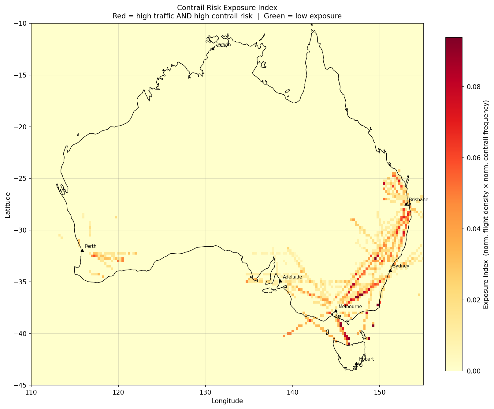
<h3 id="plot-2-exposure-index-where-avoidance-would-matter-most">Plot 2: Exposure Index: Where Avoidance Would Matter Most</h3>

<p>This plot provides an indicator of prioritisation for avoidance effort. Each grid cell is scored as: exposure = normalised_flight_density × normalised_contrail_frequency. Dark orange/red = busy AND risky.</p>

<p><img src="/assets/images/entry_5_exposure.png" alt="Contrail Exposure Index Map" /></p>

<p>This presents some interesting results where the two (contrail formation and flight density) might overlap. The peak cell was found at 36.25°S, 148.00°E with an exposure score of 0.123, which is Snowy Mountains / Monaro Tablelands and is a part of the Sydney-Melbourne route, which is the 6th most travelled route worldwide<sup><a href="#ref1">1</a></sup>!</p>

<p>Another cell of interest is 41.00°S, 146.50°E which is over the Bass Strait (flights to and from Tasmania). Its atmospheric risk is around ~3× higher than the NSW tablelands cells but fewer aircraft transit it. Northern Territory is completely blank here. Anecdotally many aircraft pass the NT on overseas flights - perhaps it is a lapse in ADS-B data.</p>

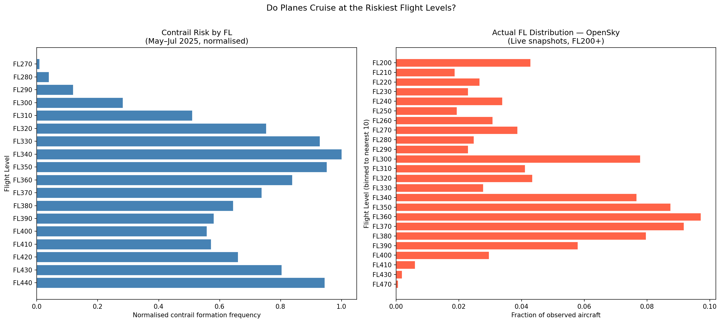
<h3 id="plot-3-altitude-alignment-are-planes-at-the-riskiest-flight-levels">Plot 3: Altitude Alignment: Are Planes at the Riskiest Flight Levels?</h3>

<p>The left plot is from last post with the different altitudes distributions shown by contrail forcing index.</p>

<p>The below FL distribution on the right comes from the 20 snapshots of OpenSky data. Each snapshot returns real-time state vector data for every transponder visible to ground receivers. One of these quantities is barometric altitude in metres, which was converted here to ft.</p>

<p>To define whether the track was airborne or not, used these two variables: 
on_ground == False and FL ≥ 200. There is nothing that identifies a climb or descent, so the distribution is more “where aircraft were observed” rather than cruising altitude.</p>

<p><img src="/assets/images/entry_5_fl_comparison.png" alt="Flight Level Comparison: Contrail Risk vs Flight Density" /></p>

<p>An observation that can be made from above is that around 93.6% of flights are observed at FL320-FL400. Even though the data is limited to 20 snapshots observed on one morning in March, aircraft cruise at certain altitudes by design, so our observations here can provide some useful indication of cruising altitude for further research while waiting for more ADSB data.</p>

<p>In earlier posts, it was observed that FL340-FL360 is where contrail risk peaks for mid-latitudes. The above right plot shows that commercial flights observed concentrate in the FL340-390 band, which has some overlap. This is significant because it relates to the potential need for changes to altitude as mentioned on Google.</p>

<h3 id="main-takeaway">Main Takeaway</h3>

<p>For the most part, there is little overlap seen here between air traffic and contrail forcing index. However, it is valuable to note the Bass Strait as one area of interest for further study on this topic.</p>

<p>At the same time, it is important to note that the data used captures a small snapshot of time and the ADSB data is even more limited, not accounting for areas such as the NT, which may potentially yield interesting results. In addition to the Bass Strait, I want to repeat the same analysis for other time periods and use more extensive data to get more insights.</p>

<hr />

<h3 id="references">References</h3>

<div class="references">
  <p><a name="ref1">[1]</a> OAG (2025). <a href="https://www.oag.com/busiest-routes-world-2025">Busiest Routes in the World 2025.</a></p>
</div>]]></content><author><name>Sidath Chandrasena</name></author><category term="Other" /><summary type="html"><![CDATA[Overlaying real ADS-B flight traffic data on contrail risk maps to find where Australia's busiest corridors intersect with high contrail forcing index values.]]></summary></entry><entry><title type="html">Entry 4: The Complex Nature of Contrails</title><link href="https://sidathchandrasena.github.io/2026/03/14/entry-4-the-complex-nature-of-contrails.html" rel="alternate" type="text/html" title="Entry 4: The Complex Nature of Contrails" /><published>2026-03-14T00:00:00+00:00</published><updated>2026-03-14T00:00:00+00:00</updated><id>https://sidathchandrasena.github.io/2026/03/14/entry-4-the-complex-nature-of-contrails</id><content type="html" xml:base="https://sidathchandrasena.github.io/2026/03/14/entry-4-the-complex-nature-of-contrails.html"><![CDATA[<figure class="banner-figure">
  <img src="/assets/images/michael-pointner-3INk5KPF1Us-unsplash.jpg" alt="An airplane flying into a golden sky at sunset" />
  <figcaption>Photo by <a href="https://unsplash.com/@pino_rumbero?utm_source=unsplash&amp;utm_medium=referral&amp;utm_content=creditCopyText">Michael Pointner</a> on <a href="https://unsplash.com/photos/an-airplane-flying-into-a-golden-sky-at-sunset-3INk5KPF1Us?utm_source=unsplash&amp;utm_medium=referral&amp;utm_content=creditCopyText">Unsplash</a></figcaption>
</figure>

<p>While looking for answers on the relationship between contrails and time of day, I stumbled across an article from science.org.</p>

<p>It<sup><a href="#ref1">1</a></sup> discusses how contrails are considered to trap large amounts of heat, which can be up to around 3x more  heat than aviation’s CO2 according to some studies. It also shares how researchers have collaborated with airlines recently to avoid contrail formation by modifying flight routes to avoid certain altitudes based on weather data, like the trial Google ran with American Airlines in 2023 with 70 flights<sup><a href="#ref2">2</a></sup> and later in 2025 in 2,400 transatlantic flights<sup><a href="#ref3">3</a></sup>.</p>

<p>The article then talks about how recent studies have identified some limitations to this approach. To summarise some of the main points:</p>

<ul>
  <li>
    <p>Small-scale trials from 2021 showed some weather models only predict where contrails form 1/5th of the time due to the contrail field being “data-starved”<sup><a href="#ref1">1</a></sup>.</p>
  </li>
  <li>
    <p>One study found over 80% of contrails in their dataset formed in existing clouds rather than in clear skies<sup><a href="#ref4">4</a></sup>. These could have a reduced warming effect, or even a cooling effect, which needs to be accounted for in contrail-avoidance schemes</p>
  </li>
  <li>
    <p>Another study found that contrail warming was not 3x that of CO2, but rather 2/3rd, suggesting a smaller impact than previously perceived<sup><a href="#ref5">5</a></sup></p>
  </li>
</ul>

<hr />
<p>To relate this back to my posts so far, in those spots such as the Southern Ocean where a high contrail forcing index is found, we should consider whether those contrails would form inside existing cloud cover, as this might cause the warming effect to be lower than the CFI values suggest.</p>

<p>My main takeaway from this article is understanding how complicated contrail formation is and how much more knowledge is needed to better understand their climate impacts, carefully balancing fuel usage and the warming impacts from each contrail region. What this means for me: it motivates me to keep analysing data in Australia, an underexplored region of the world, and share these findings.</p>

<hr />

<h3 id="references">References</h3>

<div class="references">
  <p><a name="ref1">[1]</a> Voosen, P. (2025). <a href="https://www.science.org/content/article/airplane-contrails-may-not-be-climate-villain-once-feared">Airplane contrails may not be the climate villain once feared.</a> <em>Science</em>, 390(6776).</p>
  <p><a name="ref2">[2]</a> Elkin, C., &amp; Sanekommu, D. (2023, August 8). <a href="https://blog.google/innovation-and-ai/technology/ai/ai-airlines-contrails-climate-change/">How AI is helping airlines mitigate the climate impact of contrails.</a> Google Blog.</p>
  <p><a name="ref3">[3]</a> Google Research (2026, March 19). <a href="https://blog.google/innovation-and-ai/models-and-research/google-research/contrail-avoidance-research/">Our new study explores how AI can reduce the climate impact of air travel.</a> Google Blog.</p>
  <p><a name="ref4">[4]</a> Petzold, A., Khan, N. F., Li, Y., et al. (2025). <a href="https://doi.org/10.1038/s41467-025-65532-2">Most long-lived contrails form within cirrus clouds with uncertain climate impact.</a> <em>Nature Communications</em>, 16, 9695.</p>
  <p><a name="ref5">[5]</a> Bickel, M., Ponater, M., Burkhardt, U., Righi, M., Hendricks, J., &amp; Jöckel, P. (2025). <a href="https://journals.ametsoc.org/view/journals/clim/38/8/JCLI-D-24-0245.1.xml">Contrail cirrus climate impact: From radiative forcing to surface temperature change.</a> <em>Journal of Climate</em>, 38(8), 1895–1912.</p>
</div>]]></content><author><name>Sidath Chandrasena</name></author><category term="Other" /><summary type="html"><![CDATA[Looking at an article which puts into perspective how complicated contrail-avoidance is in relation to my own observations so far with the Google dataset.]]></summary></entry><entry><title type="html">Entry 3: Contrails with Respect to Latitude, Altitude and Time</title><link href="https://sidathchandrasena.github.io/2026/03/09/entry-3-contrail-probabilities-with-respect-to-latitude-altitude-time.html" rel="alternate" type="text/html" title="Entry 3: Contrails with Respect to Latitude, Altitude and Time" /><published>2026-03-09T00:00:00+00:00</published><updated>2026-03-09T00:00:00+00:00</updated><id>https://sidathchandrasena.github.io/2026/03/09/entry-3-contrail-probabilities-with-respect-to-latitude-altitude-time</id><content type="html" xml:base="https://sidathchandrasena.github.io/2026/03/09/entry-3-contrail-probabilities-with-respect-to-latitude-altitude-time.html"><![CDATA[<p>In Entry 2, I looked at where contrails form and at what altitudes in Australia during winter months.</p>

<p>I saw that the contrail forcing index was significantly higher over the Southern Ocean (area from Australia’s southern coast to Antarctica) which was interesting given the little aviation traffic there. However, it is important to keep in mind that the dataset only indicates the contrail forcing index and does not indicate whether any aircraft flew there.</p>

<p>In this post, I will re-examine these plots, but see if I can gain further insight by breaking the plots down in terms of latitude, flight level and time of day.</p>

<p><em>Please note that the below plots refer to the CFI as “probability” and could not be regenerated to update the accurate naming because the data was originally stored in a local database.</em></p>

<hr />

<p>Plots 1 and 2 are heatmaps which aggregate the data to compare Mean Contrail Forcing Index and Contrail Frequency (created in Entry 2) against latitude values. The following table gives some context on latitude values:</p>

<table>
  <thead>
    <tr>
      <th>Latitude</th>
      <th>Geography</th>
    </tr>
  </thead>
  <tbody>
    <tr>
      <td>45°S</td>
      <td>Deep Southern Ocean — no land, no flights</td>
    </tr>
    <tr>
      <td>43°S</td>
      <td>Southern Tasmania (Hobart)</td>
    </tr>
    <tr>
      <td>38°S</td>
      <td>Southern Victoria coast — aviation zone boundary (dashed white line)</td>
    </tr>
    <tr>
      <td>35°S</td>
      <td>Sydney / Canberra</td>
    </tr>
    <tr>
      <td>32°S</td>
      <td>Perth</td>
    </tr>
    <tr>
      <td>27°S</td>
      <td>Brisbane</td>
    </tr>
    <tr>
      <td>25°S</td>
      <td>Tropic of Capricorn boundary — transition to tropical atmosphere</td>
    </tr>
    <tr>
      <td>23°S</td>
      <td>Alice Springs</td>
    </tr>
    <tr>
      <td>17°S</td>
      <td>Darwin / north Kimberley</td>
    </tr>
    <tr>
      <td>10°S</td>
      <td>Northern edge of the data domain, above Cape York</td>
    </tr>
  </tbody>
</table>

<p><br /></p>
<h3 id="plot-1-mean-contrail-forcing-index-by-flight-level--latitude">Plot 1: Mean Contrail Forcing Index by Flight Level &amp; Latitude</h3>
<p><img src="/assets/images/entry_4_alt_lat_mean.png" alt="Mean Contrail Forcing Index by Flight Level and Latitude" /></p>

<p><br /></p>
<h3 id="plot-2-contrail-frequency-by-flight-level--latitude">Plot 2: Contrail Frequency by Flight Level &amp; Latitude</h3>
<p><img src="/assets/images/entry_4_alt_lat_freq.png" alt="Contrail Frequency by Flight Level and Latitude" /></p>

<p>Plots 1-2 give some helpful insight by adding flight altitudes in addition to location. It appears that as you move north, the contrail-favourable layer is at higher altitudes. For example, at southern latitudes, we have a peak CFI of 0.13-0.15 at FL330–FL350, at mid latitudes, the peak shifts slightly to FL340-360, and in the tropical north, the contrail favourable layer appears at FL380-FL440.</p>

<hr />
<p>In addition to altitudes, I can also look at how the time of day may change the level of contrail risk:</p>

<p><br /></p>
<h3 id="plot-3-overall-diurnal-signal">Plot 3: Overall Diurnal Signal</h3>
<p><img src="/assets/images/entry_4_diurnal_overall.png" alt="Overall Diurnal Contrail Signal" /></p>

<p>As can be seen above, there are noticeable differences in the bar plots so conditions are not uniform in time, with contrail forcing index highest at around 14 UTC, which is around 00:00 AEST (midnight).</p>

<p><br /></p>
<h3 id="plot-4-diurnal-signal-by-latitude-band">Plot 4: Diurnal Signal by Latitude Band</h3>
<p>I can also further examine the results of this bar plot by splitting it into different latitudes as discussed above:
<img src="/assets/images/entry_4_diurnal_by_band.png" alt="Diurnal Contrail Signal by Latitude Band" /></p>

<p>Both plots reveal 14 UTC (midnight AEST) to be the peak, with the Southern Ocean band dominating by 3-7x at every UTC hour, and with 02 UTC (Noon AEST) as the trough.</p>

<p><br /></p>
<h3 id="the-main-takeaway">The main takeaway</h3>
<p>From what I have, I observed that contrail formation conditions are the highest overnight and lowest around midday. How does this compare to what is mentioned online?</p>

<p>It was found that the season with the highest amount of contrails is winter in a study taken in the Northern Hemisphere<sup><a href="#ref1">1</a></sup>, which is when this dataset was recorded. Early morning flights tend to create “cooling contrails”, while evening and night flights produce contrails with the highest warming contribution.<sup><a href="#ref2">2</a></sup> This demonstrates how contrail formation conditions do not necessarily equate to high amounts of warming.</p>

<hr />

<h3 id="references">References</h3>

<div class="references">
  <p><a name="ref1">[1]</a> Stuber, N., Forster, P., Rädel, G., et al. (2006). <a href="https://doi.org/10.1038/nature04877">The importance of the diurnal and annual cycle of air traffic for contrail radiative forcing.</a> <em>Nature</em>, 441, 864–867.</p>
  <p><a name="ref2">[2]</a> Transport &amp; Environment — <a href="https://www.transportenvironment.org/articles/contrail-avoidance">Contrail Avoidance</a></p>
</div>]]></content><author><name>Sidath Chandrasena</name></author><category term="Other" /><summary type="html"><![CDATA[Breaking down contrail forcing index by latitude, flight level, and time of day with interesting observations in the Southern Ocean.]]></summary></entry></feed>