Entry 2: Database Migration and Starting Geospatial Analysis
So far, I’ve been using a local SQLite database imported from Google Contrails API to store my week’s worth of data to take a first glimpse. As I thought of making my dataset bigger, I started thinking of better ways to store this data.
I decided to migrate the database to PostgreSQL with Docker Desktop, which I am already familiar with and will be more efficient at running queries with big datasets.
Since migrating the database to Postgres, here is a summary of it now. As you can see, data is restricted to the Australian continent:
| Dimension | Detail |
|---|---|
| Period | 15 May 2025 20:00 UTC → 14 July 2025 14:00 UTC (~60 days) |
| Interval | Exactly 6 hours — no gaps |
| Snapshots | 239 timestamps (02:00, 08:00, 14:00, 20:00 UTC each day) |
| Total rows | ~109.8 million |
| Latitude | −45° to −10° · 141 values · 0.25° steps |
| Longitude | 110° to 155° · 181 values · 0.25° steps |
| Coverage | Australia only — no global data |
| Flight levels | FL270 to FL440 · 18 levels · FL10 steps |
| Grid completeness | 141 × 181 × 18 × 239 = fully consistent, no missing cells |
Looks ready for some more analysis!
Analysis
Now we have around 2 months’ worth of data, we can look into contrail formation in Australia during the winter period.
From an initial look at the dataset, it was found that 97.1% of contrails values were found to be zero. It is important to note here that the contrails variable is an output from the Google Contrails API that is not measured data, but rather an index that comes from a combination of satellite observations, ML model’s output, ECMWF HRES forecast data and CoCiP (Contrail Cirrus Prediction)1. So this may reflect the model’s limitations in data-sparse regions rather than the actual atmospheric conditions.
To get more meaningful results from the data, two variables were created to quantify the frequency and intensity of contrails.
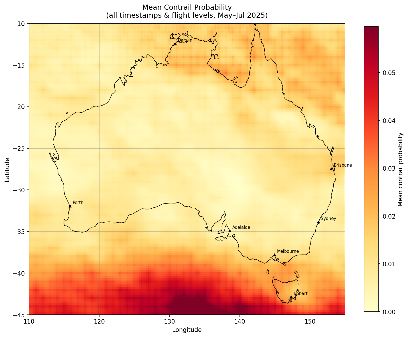
Mean contrail forcing index: For each map “cell”, the average CFI is calculated across different timestamps and flight levels. These rows include CFI values of zero as well.
Contrail Frequency: A binary flag per row which returns 1 if CFI > 0 and 0 if not, which is then averaged within groups. Answers question of: what fraction of timestamp-flight level combinations are contrail-forming?
These 2 variables were then represented spatially using GeoPandas, shapefiles of Australia and coordinates of major cities using the longitudes & latitudes, resulting in these plots:
Please note that the below plots refer to the CFI as “probability” and could not be regenerated to update the accurate naming because the data was originally stored in a local database.
Plot 1: Mean Contrail Forcing Index
Plot 2: Contrail Frequency
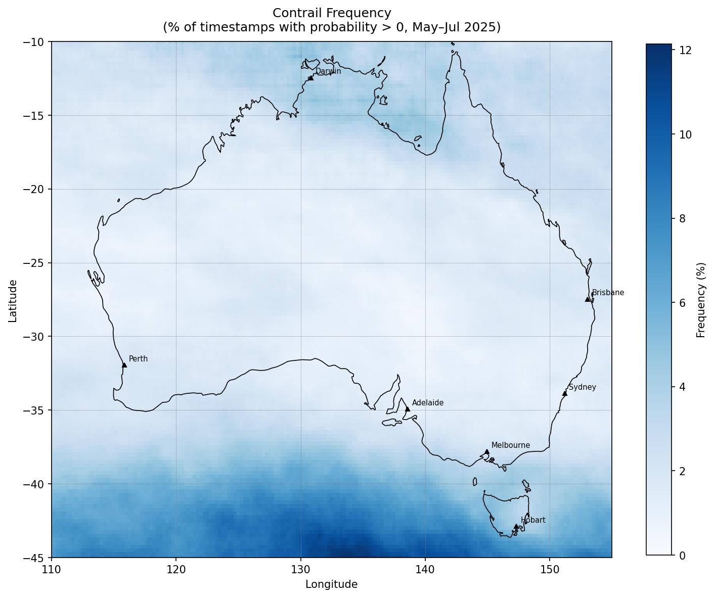
Plots 1 and 2 show that both strength and frequency of contrail formation are concentrated towards the south of the continent, with some interesting activity in the North to a lesser extent.
Plot 3: Altitude Profile
Shows contrail formation likelihood across the 18 flight levels in Contrails API dataset:
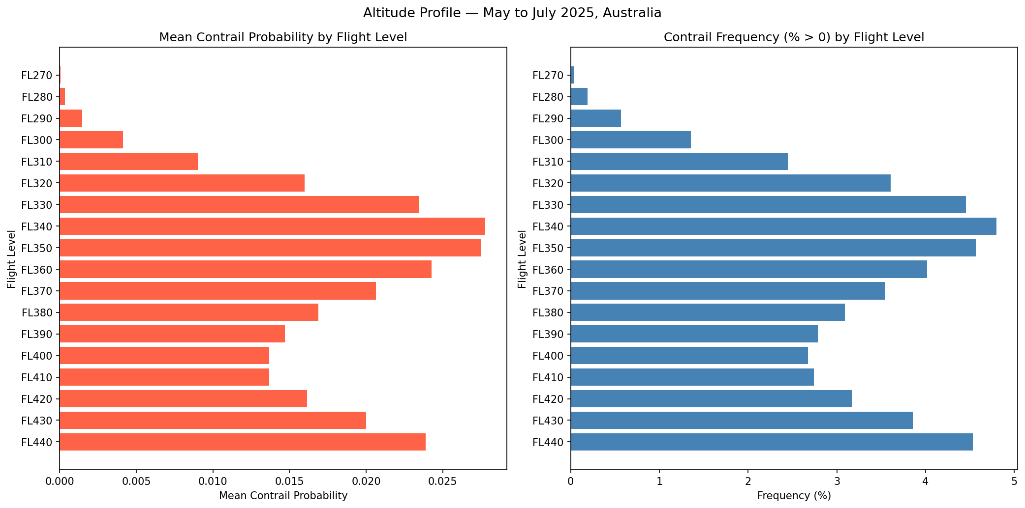
Between FL270-FL440, notable altitudes for contrail frequency and intensity appear to be at FL330 (33,000 ft), FL340 (34,000 ft), FL350 (35,000 ft) and FL440 (44,000 ft).
Plot 4: Hotspot Maps by Flight Level Band
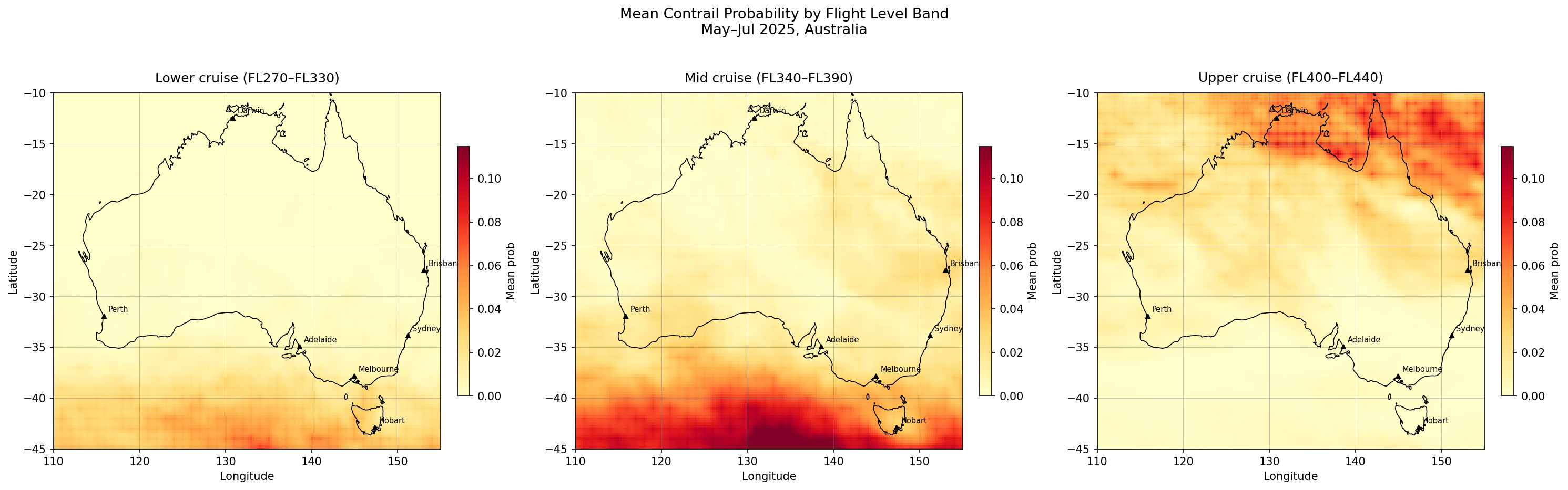
The above is probably the most interesting plot in my opinion. It reveals that the hotspot locations are altitude dependent, with higher likelihood for contrail formation over the Southern Ocean south of the mainland at a mid-cruise altitude (34-39,000 ft) while higher concentrations near Darwin and Northern Queensland are at an upper cruising altitude between 40-44,000 ft. This suggests that any avoidance strategy would need to vary based on the region it’s in.
References
[1] Google for Developers. Contrails API: forecast description.